9 · Was the battery well traded? A backtesting framework

Intermediate Production Case B Backtesting MPC

In this chapter

• Build a backtest that cannot cheat: policies see only what was known at the time (information_policy="historical_only"), and asking for the future raises an error
• Benchmark against perfect foresight, fairly, by valuing the energy left in the battery at the end, and read the capture ratio
• Compare policies: greedy thresholds, rolling-horizon model predictive control (MPC) as a schedule or as a bid, and ten price bands set the day before
• Model network constraints that leave the battery constrained on to charge at $10,000/MWh, and the constraint management that avoids it
• Attribute the gap to its causes with counterfactuals, and see why the answer depends on the order unless you use Shapley values

Chapter 2 optimised a battery with perfect knowledge of prices. Real batteries are traded through bids submitted before prices are known, behind network constraints, by software that re-plans every few minutes. The owner's question is not "what is optimal?" but "how well did we do, and where did the rest go?" A backtest answers it, if it is honest about what was known when. This chapter builds one and uses it. It is Milestone 7 of the book: the common backtesting framework later chapters reuse.

---

1 · The real-world problem

A battery operator's monthly report (the pattern here is drawn from real ones) lists revenue by market, cycles and throughput margin. Then come the questions:

• The battery was constrained on to charge at about $10,500/MWh on the same day it captured a $14,000 spike. How much did that cost, and how do we stop it?
• It was empty before the evening peak several times. Bad forecasting, bad bidding, or bad luck?
• One price band sat in the mid-$80s while the market cleared at $50–60. How much did stale bands cost?
• Is a 60 % capture ratio good?

2 · The physical system

The Case B battery: 10 MW / 20 MWh, 3–97 % SOC window, ≈ 88 % round-trip efficiency, and a wear cost of $40/MWh discharged (Chapter 2; Chapter 10 revisits it). It trades energy and ten FCAS markets, including the very fast 1-second services introduced in October 2023.

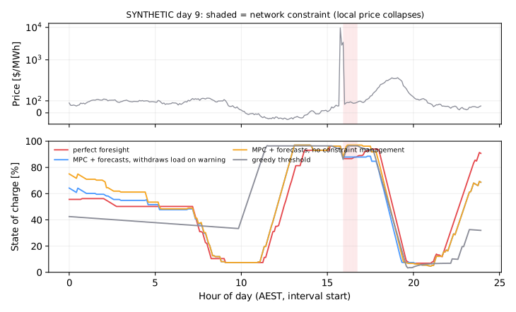
The market is a synthetic month, calibrated to a confidential source: a NEM battery operator's reports. It has 5-minute prices with a solar trough, morning and evening peaks and spikes of up to $15,000/MWh. LOWER1SEC is valuable through the day and collapses in the evening peak. Network constraint events cluster at 17:00–19:00. During an event the battery's local price falls below −$1,000: it cannot be dispatched to generate, and if it offers load it is constrained on, charging at the regional price whatever that is.

3 · The decision being judged

A trading policy: every 5 minutes, the offers the battery submits. These are a price–volume staircase for generation, another for load (as in Chapter 8), and FCAS enablement. The market then decides what is dispatched.

4 · The framework: forecast, decide, settle

The framework keeps the book's three-way separation explicit in code:

Piece	Code	Rule
What could be known	MarketView(market, t, information)	Past outcomes; forecasts issued at t; constraint warnings
What was decided	Policy.decide(view, soc) → Instruction	Offers and FCAS for interval t
What happened	run_backtest(policy, market, spec, start, end)	Dispatch at actual prices and constraints, physics, settlement

Under historical_only, the view hands a policy past prices and forecasts issued at decision time. These are a pre-dispatch-like price forecast whose error grows with lead time and which sees only half the spikes, and only shortly before. It also gets a constraint warning that catches three events in four. Asking for a future outcome raises LookAheadError. Only a benchmark labelled perfect_foresight may read the future, and its results carry the label.

Look-ahead bias is the backtest's original sin

Using today's price to decide today's bid, re-fitting a model on data that includes the test period, or setting bands from a month that includes the day being traded: each makes a strategy look better than it can be. The framework makes the honest path the easy one. daily_bands uses only the days before, and a test changes the future and checks that nothing a historical policy sees changes with it.

Settlement. Energy is settled at the regional price and FCAS at the enablement price. Dispatch follows the offers, local constraints override them, and the state of charge must stay inside the window. This is a simplified dispatch, not NEMDE.

5 · The benchmark: perfect foresight, fairly

The ceiling is one LP over the whole window with the actual prices: Chapter 2's energy + FCAS model, now with ten markets and the constraint events.

Policies end the window with different amounts of energy stored. A policy that sells its inventory on the last day looks better than one that doesn't, without having traded better. So every result is scored on adjusted profit:

\[ \Pi^\text{adj} = \text{revenue} - k_{deg}\,\text{MWh}_\text{discharged} + v\,\big(\text{SOC}_\text{end} - \text{SOC}_\text{start}\big), \]

with one inventory value \(v\) for everyone (the window's mean price × η). The benchmark LP values its own end-of-window energy at the same \(v\). That makes it a true upper bound on every policy's adjusted profit (a tested property). The capture ratio is \(\Pi^\text{adj}/\Pi^\text{adj}_\text{PF}\).

6 · The policies

• Greedy threshold. Charge below $40, discharge above $150, offer all FCAS. This is common, and the source of the "empty before the peak" pattern.
• Rolling MPC. Every hour, re-solve the energy + FCAS LP over the next 24 hours on the forecasts, then act. The plan must end at 50 % SOC, and the controller doesn't plan to discharge, and withdraws its load offer, when a constraint is warned.
• As a schedule: deliver the planned MW at any price.
• As a bid: offer the planned volume at the price the plan's own dual says it is worth. The value of stored energy \(\lambda_t\) gives a discharge threshold \(\lambda_t/\eta_d + k_{deg}\) and a charge threshold \(\lambda_t\eta_c\). The rest of the inverter is offered at a spike price, to catch spikes the forecast missed. The real price then decides.
• Bands. Bid MPC, but each threshold snaps to one of ten band prices set the day before (Chapter 8's rule). Two variants: a stale set chosen once (with a band at $85), and bands re-calibrated daily from quantiles of the past fortnight's prices.

7 · Results

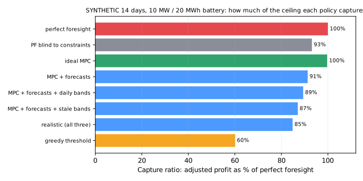
Fourteen synthetic days (days 8–21 of the month), the same battery and the same prices throughout:

Policy	Adjusted profit	Capture	Cycles	Throughput margin	Forced-charge cost
Perfect foresight	$199,332	100 %	22.1	$491/MWh	$0
Ideal MPC (perfect forecasts, any price)	$198,671	99.7 %	21.9	$494/MWh	$0
MPC + forecasts	$181,995	91.3 %	20.9	$477/MWh	$998
MPC + forecasts + daily bands	$178,146	89.4 %	18.6	$521/MWh	$998
MPC + forecasts + stale bands	$173,524	87.1 %	17.4	$540/MWh	$998
MPC + forecasts + stale bands, no constraint management	$169,071	84.8 %	18.4	$499/MWh	$7,884
Greedy threshold	$119,830	60.1 %	35.0	$212/MWh	$8,119

Planning around the constraints matters even with perfect foresight. The same LP, blind to the constraint events, earns $185,610 (93.1 %). It plans to charge in intervals where it is then forced to, and to discharge where it can't, and pays $7,963 in forced charging. The $998 that even the constraint-managed controllers pay comes from the one event in four that arrives without a warning.

What the table says:

1. Re-planning is nearly free; forecasting isn't. A 24-hour rolling horizon with perfect forecasts loses only 0.3 % against hindsight over the whole fortnight. The receding horizon is not the problem. Forecast error costs ≈ 8.4 points.
2. Greedy trades twice as much for less. Thirty-five cycles at a $212/MWh margin, against eighteen at about $500. A fixed threshold sells into any price above $150 and has nothing left when the real spikes come. More cycling is not more value.
3. Constraint management is worth real money. Withdrawing the load offer when a constraint is warned turns $7.9k of forced charging into about $1k. The warning misses a quarter of events.
4. A 60 % capture ratio is not "good". It depends entirely on the benchmark and the window. Against an honest benchmark, a competent controller here captures 85–91 %, and the greedy rule captures 60 %.

FCAS earns about two-thirds of revenue under every policy that offers it, consistent with the real battery behind the calibration.

8 · Where did the money go? Counterfactual attribution

Start from the ideal controller and switch on one imperfection at a time: forecasts instead of hindsight, stale bands, no constraint management. Three switches make \(2^3 = 8\) backtests:

Imperfections switched on	Adjusted profit
none (ideal controller)	$198,671
no constraint management	$191,609
stale bands	$186,951
forecasts	$181,995
stale bands + no constraint management	$180,967
forecasts + no constraint management	$176,329
forecasts + stale bands	$173,524
all three	$169,071

The total loss is $29,600. How much of it is "due to" each cause? The usual answer is a waterfall: add the causes in some order and record each step. But the causes interact. Stale bands cost $11,700 on top of perfect forecasts, but only $8,471 once forecasts are already wrong: the forecast error had already caused some of the same misses. So the waterfall depends on its order.

Shapley values remove the arbitrariness. Each cause gets its marginal loss averaged over every order in which the causes could be added:

\[ \phi_i = \sum_{S \subseteq N\setminus\{i\}} \frac{|S|!\,(n-|S|-1)!}{n!}\,\big(v(S\cup\{i\}) - v(S)\big), \qquad \sum_i \phi_i = v(N) - v(\varnothing). \]

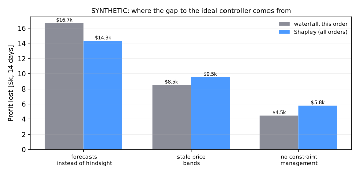
Cause	Waterfall (forecast → bands → constraints)	Shapley
Forecasts instead of hindsight	−$16,676	−$14,308
Stale price bands	−$8,471	−$9,512
No constraint management	−$4,453	−$5,780
Total	−$29,600	−$29,600

Both add up to the same total, but they split it differently. The waterfall blames whatever comes first, and Shapley shares the interactions fairly. Report Shapley values, and say which counterfactuals defined the game.

The operator's checklist, as code

Each pattern from the operator reports becomes a check on the ledger:

• SOC at each day's peak-price interval (soc_at_daily_peak)
• MWh missed in spike intervals while energy was available (spike_mwh_missed)
• Forced-charge cost
• Revenue per cycle

Each becomes an alert in production.

Why these techniques?

Why these techniques? Structure → method

Property of the problem	Here	So
Question	would a policy have made money using only what was known at the time?	a backtest that cannot look ahead: MarketView raises LookAheadError
Information	prices, forecasts and constraint warnings arrive over time	rolling-horizon MPC: re-solve every hour, commit only the first step
Per-step model	linear profit, battery energy balance, ten FCAS markets	an LP of about 3,700 variables, solved in well under a second
Time coupling	state of charge links every interval	plan over 24 hours, and end the plan at 50 % SOC so it stays feasible
Benchmark	no policy can beat hindsight, but end inventory differs between policies	one LP over the window with the actual prices, valuing end energy at the same \(v\)
Causes of loss	forecasts, stale bands and constraint management, which interact	\(2^3 = 8\) counterfactual backtests, then Shapley values
Cost	336 LPs per backtest; 8 backtests for attribution	a few minutes in total

Chosen. - Rolling-horizon MPC matches how the information arrives. Each hour the plan is rebuilt on the newest forecast; only the first step is acted on. The LP's dual \(\lambda_t\) on the energy balance then gives the bid thresholds. - A perfect-foresight LP as the ceiling, with a common inventory value, so adjusted profit compares like with like. - Shapley values share a total that depends on the order in which causes are added. Each cause gets its marginal loss averaged over all orders.

Not chosen. - One full-window optimisation as the policy. It uses future prices. It is the benchmark, and its results carry the label. - Dynamic programming over state of charge. It is exact for one battery, but the action space spans ten markets and gives no duals for bidding; the LP does both. - A stochastic programme at every step. Closer to reality, but scenario trees grow quickly, and the receding horizon already re-plans hourly. Chapter 15 treats the commitment decision where it matters. - A waterfall attribution. It adds causes in one order and blames whichever comes first; here stale bands cost $11,700 alone but $8,471 after forecasts.

What the theory guarantees. - Perfect foresight is an upper bound on every policy's adjusted profit, because every policy's schedule is feasible in that LP. Receding horizon has no general optimality guarantee; the fixed end SOC gives feasibility, and the 0.3 % loss against hindsight is measured, not proved. - Shapley's value is the only attribution that is efficient, symmetric, additive and gives nothing to a cause with no effect, and it sums exactly to the total loss.

References. - Rawlings, Mayne and Diehl (2017), Model Predictive Control: what is re-solved, what is committed, and when it is stable (Chapter 9). - Shapley (1953), A value for n-person games: the axioms behind the attribution (Chapter 9). - Hyndman and Athanasopoulos (2021), Forecasting: Principles and Practice: time-series cross-validation as an honest backtest (Chapter 4). - Choosing a technique for how time and information choose between a single solve and a rolling one.

9 · Implementation

from energy_or.backtest import (
    PerfectForesight,
    RollingMPC,
    attribute_losses,
    kpis,
    run_backtest,
)
from energy_or.bess import BatterySpec
from energy_or.data.bess_market import bess_market

market = bess_market()  # SYNTHETIC month
spec = BatterySpec(
    energy_mwh=20.0, eta_charge=0.94, eta_discharge=0.94, degradation_cost_per_mwh=40.0
)
start, end = 7 * 288, 21 * 288
v = float(market.rrp_per_mwh[start:end].mean()) * spec.eta_discharge

pf = run_backtest(
    PerfectForesight(spec, start, end, inventory_value_per_mwh=v), market, spec, start, end
)
mpc = run_backtest(RollingMPC(spec, resolve_every=12, bands="daily"), market, spec, start, end)
print(kpis(mpc, pf, v).capture_ratio)
attr = attribute_losses(market, spec, start, end, v)  # 8 backtests
print(attr.shapley)

10 · Solve: what it costs to run

Perfect foresight is one LP with about 52,000 variables, solved in ≈ 2 s by HiGHS. Each MPC backtest is 336 LPs of about 3,700 variables, ≈ 45 s for the fortnight. The attribution's eight backtests take ≈ 6 minutes. A 5-minute production cycle has room for one MPC solve in well under a second.

11 · Interpret

For the owner:

• Of a $199k ceiling, a realistic controller earns $169k. Of the $30k gap:
• $14k is forecasting. Better forecasts help, but only so far.
• $10k is stale bands. Re-calibrate the bands deliberately, and test the change with this framework first, because re-calibration can also make things worse.
• $6k is constraint management.
• Better forecast accuracy is not the goal; decision value is. The attribution measures forecast error in dollars, not in MAE.

12 · Backtest the backtest

A backtest is a model too. Check it the way the tests do:

• the perfect-foresight replay must reproduce its own LP to the cent;
• no policy may beat the benchmark;
• physics and FCAS headroom must hold for any policy, however silly;
• a historical policy's view must be unchanged when the future is changed.

13 · Adding realism

• Price impact. A 10 MW battery rarely moves the regional price, but it does set prices in thin FCAS markets. Perfect foresight overstates the ceiling there.
• Rebid timing and gate closure. Offers are locked shortly before each interval. Model the lag between decision and dispatch.
• Causer pays, regulation utilisation, FCAS trapezia. These are all simplified here.
• Telemetry vs calculated SOC. In the incident lab, the battery's reported SOC drifts from the energy balance and the controller plans on the wrong number.

14 · Exercises

Guided

For a two-day window, compute the capture ratio of the greedy policy with and without the inventory adjustment. Which way does the adjustment move it, and why?

Engineering

Add a "late file" incident: on one day the forecast is issued two hours stale. Measure the cost in the attribution framework as a fourth factor (16 backtests).

Market

Lower the stale band set's $85 band to $55 and re-run. How much of the band loss does one band explain?

Challenge

Prove that Shapley values are the only attribution that is efficient, symmetric, additive and gives zero to a factor that never changes the outcome.

Production challenge

Turn the ledger into a daily report: capture ratio, revenue by market, forced charging, SOC at peak, spike MWh missed. Decide the alert thresholds, and where the report runs (Cloudflare Worker + R2, later chapters).

15 · Production perspective

• The backtester and the live system share code. The same Policy object runs in both. Only the view changes: historical data replay or live feeds.
• Every result carries its information policy. A dashboard must never show a perfect-foresight number without saying so.
• Attribution is the monthly conversation with the trader. It is in dollars, by cause, with the counterfactuals written down.

Run it yourself

Artefact	Location
Views, instructions, simulator, ledger	src/energy_or/backtest/framework.py
Policies (perfect foresight, rolling MPC, bands, greedy)	src/energy_or/backtest/policies.py
KPIs and pattern checks	src/energy_or/backtest/metrics.py
Counterfactual and Shapley attribution	src/energy_or/backtest/attribution.py
Synthetic market month	src/energy_or/data/bess_market.py
Tests	tests/test_backtest.py
Notebook	notebooks/09_backtesting_a_battery.ipynb