T0 · The simplex method by hand: walking the corners of Case A
Foundation Optimisation toolbox Case A Simplex · big-M · two-phase · Bland

In this chapter
- Why the graphical method of Chapter 1 stops at two decision variables, and what replaces it
- Put Case A into standard form with slack variables, then solve it by hand in two pivots, reading the shadow prices from the final tableau
- Handle ≥ and = constraints with surplus and artificial variables, by the big-M and two-phase methods, and see how infeasibility shows itself
- Watch the textbook rule cycle at a degenerate corner, and Bland's rule fix it
- Know what HiGHS does differently, and why you will almost never pivot by hand again
Chapter 1 drew the feasible region and slid the objective line until it touched the last corner. That works because the picture has two axes, one for each decision. A battery's day (Chapter 2) has 288 dispatch decisions. Chapter 15's commitment problem has 144,002. Nobody can draw a 144,002-dimensional polygon, but the idea survives: an LP's optimum is at a corner, and from any corner you can move along an edge to a better neighbouring corner until no neighbour is better. That walk is the simplex method (Dantzig, 1963). This chapter does it by hand once, so that a solver's output (basis, reduced costs, duals, "infeasible") always means something to you.
Why these techniques? Structure → method
| Property of the problem | Here | So |
|---|---|---|
| Objective and constraints | linear | the optimum (if one exists) is at a corner of the feasible region: search corners only |
| Number of decision variables | 2 in Case A; 288 in a battery day; 144,002 in Chapter 15 | graphical method only for 2 (or 3); otherwise an algebraic method |
| Constraint types | ≤ (Case A); ≥ and = (contract minimums, a line that must be full) | ≤ adds a slack and gives a starting corner for free; ≥ and = need artificial variables and the big-M or two-phase method |
| Degeneracy | several constraints can meet at one corner (ties in the ratio test) | a pivot rule that cannot cycle (Bland) |
| Size in practice | thousands to millions of variables, sparse | revised simplex or interior-point methods in a solver (HiGHS), never a dense hand tableau |
Chosen. - The tableau simplex method, because every quantity a solver reports is visible in it: - the basis (which variables are free to move); - the reduced costs (would bringing a variable in help?); - the minimum-ratio test (how far can we move before leaving the feasible region?); - the duals in the objective row, which are the shadow prices of Chapter 1. - Big-M and two-phase as the two standard ways to start when the origin is not feasible. - Bland's rule to show that cycling is real and avoidable.
Not chosen. - The graphical method beyond two variables: there is no picture to draw. - Enumerating every corner: a problem with \(n\) variables and \(m\) constraints can have up to \(\binom{n+m}{m}\) corners, astronomically many. The simplex method visits a tiny fraction of them, because each pivot improves the objective. - Interior-point methods by hand (Karmarkar, 1984). They are polynomial in the worst case and excellent for very large LPs, but they cross the inside of the region, so they do not teach the corner and basis vocabulary. HiGHS offers both.
What the theory guarantees. - If an LP has an optimum, one is at a corner (a basic feasible solution). - The simplex method with an anti-cycling rule finds it in finitely many pivots, or proves the problem unbounded or infeasible. - At the optimum, the objective-row entries under the slack columns are the dual values (shadow prices), and strong duality makes the primal and dual objectives equal. - The worst case is exponential (Klee and Minty, 1972), but typical problems need a number of pivots roughly proportional to the number of constraints.
References. Dantzig (1963), Linear Programming and Extensions; Charnes (1952) on big-M and degeneracy; Bland (1977) on finite pivoting rules; Klee and Minty (1972) on the worst case; Karmarkar (1984) on interior-point methods; Bertsimas and Tsitsiklis (1997), chapters 2–4. All are in Further reading.
1 · Standard form: turning inequalities into equalities
Case A from Chapter 1:
The algebra needs equalities, so give each \(\le\) constraint a slack variable: the part of the right-hand side left unused.
Each slack means something physical: - \(s_1\) is spare line capacity [MW]; - \(s_2\) and \(s_3\) are the wind each farm has available but does not export.
| Constraint type | Add | Meaning | Gives a starting corner? |
|---|---|---|---|
| \(\le\) | slack \(s \ge 0\) | unused capacity | yes: \(s = b\) |
| \(\ge\) | minus a surplus \(e \ge 0\), plus an artificial \(a \ge 0\) | excess over the minimum | no: the surplus enters with −1, so an artificial is needed |
| \(=\) | an artificial \(a \ge 0\) | none: it must end at zero | no |
2 · The first tableau
Write the constraints as rows, and the objective as \(z - 50P_A - 80P_B = 0\) in the last row. Every slack column is a column of the identity matrix, so the slacks form the first basis. The starting corner is \(P_A = P_B = 0\), \(s = (100, 70, 80)\): export nothing.
Optimality test (maximisation): if any entry of the z row is negative, increasing that variable increases \(z\), so the corner is not optimal. Here both \(-50\) and \(-80\) are negative.
3 · Pivot 1: who enters, who leaves
- Entering variable (Dantzig's rule): the most negative z-row entry, \(-80\), so \(P_B\) enters. Each MW of WF_B adds $80 an hour, the steepest improvement.
- Leaving variable (minimum-ratio test): divide each right-hand side by the entering column's positive entries: \(s_1\): 100/1 = 100, \(s_3\): 80/1 = 80 (\(s_2\) has 0 in that column, so it is no limit). The smallest ratio, 80, means WF_B's availability binds first, so \(s_3\) leaves. Choosing anything larger would push \(s_3\) negative, that is, export more wind than exists.
- Pivot: divide the \(s_3\) row by its pivot entry (1), then subtract multiples of it from every other row to clear the \(P_B\) column.
New corner: \(P_A = 0, P_B = 80\), $6,400 an hour. Still a \(-50\) in the z row.
4 · Pivot 2 and the optimum
\(P_A\) enters. Ratios: \(s_1\): 20/1 = 20, \(s_2\): 70/1 = 70, so \(s_1\) leaves, and the shared line fills.
No negative entries remain: optimal at \(P_A = 20\), \(P_B = 80\), $7,400 an hour. This is Chapter 1's answer, reached by two moves along the edges of the feasible region. The final z row also contains Chapter 1's shadow prices:
| Column | z-row entry | Meaning |
|---|---|---|
| \(s_1\) (shared line) | 50 | one more MW of line is worth $50 an hour: WF_A's value, since WF_A is the farm curtailed |
| \(s_2\) (WF_A's wind) | 0 | WF_A has 50 MW spare (\(s_2 = 50\)); more wind is worth nothing |
| \(s_3\) (WF_B's wind) | 30 | one more MW of WF_B's wind is worth $80 − $50 = $30: it displaces a WF_A MWh |
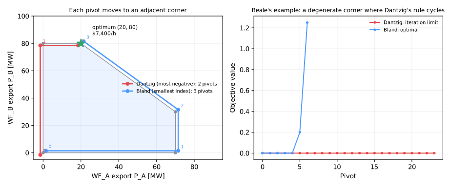
The entering rule chooses the path, not the destination. Bland's rule (smallest index) brings in \(P_A\) first and takes three pivots, (0,0) → (70,0) → (70,30) → (20,80), to the same optimum.
5 · When the origin is not feasible: big-M and two-phase
Add two realistic conditions. The network asks for the line to be full (\(P_A + P_B = 100\)), and WF_A's offtake contract has a minimum of 30 MW (\(P_A \ge 30\)). Now \(P_A = P_B = 0\) is not feasible, so there is no free starting corner. Standard form:
The artificials \(a_1, a_2\) make an identity basis, but they are not real: a solution is only valid once both are zero. There are two standard ways to get there:
- Big-M (Charnes, 1952): give each artificial a huge penalty, (\max\; 50P_A + 80P_B
- M a_1 - M a_2). Any solution with an artificial still positive loses so badly that the simplex method drives the artificials out first. The risk is numerical: M must be large enough to dominate, yet small enough not to swamp the real coefficients in floating point.
- Two-phase: Phase 1 ignores the real objective and minimises \(a_1 + a_2\). If the minimum is above zero, no feasible point exists, and the problem is reported infeasible. If it is zero, the final Phase 1 corner is feasible, and Phase 2 optimises the real objective from there. Solvers use this approach (or variants of it), because it avoids choosing M.
Two-phase on this problem (simplex(..., method="two_phase")):
phase 1 (start: minimise a1 + a2 = 130)
basis  P_A  P_B  e2  s3  s4  a1  a2   rhs
   a1    1    1   0   0   0   1   0   100
   a2    1    0  -1   0   0   0   1    30
   s3    1    0   0   1   0   0   0    70
   s4    0    1   0   0   1   0   0    80
    z   -2   -1   1   0   0   0   0  -130      → P_A enters, a2 leaves; then P_B enters, a1 leaves

phase 2 (artificials gone; real objective)
basis  P_A  P_B  e2  s3  s4  a1   a2   rhs
  P_B    0    1   1   0   0   1   -1    70
  P_A    1    0  -1   0   0   0    1    30
   s3    0    0   1   1   0   0   -1    40
   s4    0    0  -1   0   1  -1    1    10
    z    0    0  30   0   0  80  -30  7100      optimal (artificial columns can no longer enter)
Optimal at \(P_A = 30\), \(P_B = 70\), $7,100 an hour; big-M gives the same answer. The duals: - the full-line equality is worth $80/MW: one more MW of line goes to WF_B; - the 30 MW minimum has dual −$30/MW: each extra MW the contract forces on WF_A costs $80 − $50. The dual of a \(\ge\) row in a maximisation is \(\le 0\).
Infeasible. Ask for \(P_A \ge 30\) and \(P_B \ge 80\) with \(P_A + P_B \le 100\): Phase 1 stops with \(a_1 + a_2 > 0\), and big-M ends with an artificial still in the basis. The two contract minimums need 110 MW of a 100 MW line, and Chapter T2's IIS would name those three rows. Unbounded. If no constraint limits an improving direction, the entering column has no positive entry, the ratio test has nothing to divide, and the method stops: there is no optimum to find.
6 · Degeneracy and cycling
A corner is degenerate when a basic variable is zero, so that more constraints than necessary meet there. A pivot from such a corner can move zero distance, and with Dantzig's rule and an unlucky tie-break the method can return to a basis it has already visited and loop for ever. Beale's classic example does exactly this (right panel of the figure: 24 pivots, objective stuck at 0). Bland's rule always picks the smallest-index candidate, both for entering and for leaving, and provably never cycles. Here it reaches the optimum, 1.25, in 6 pivots. Production solvers use perturbation and other safeguards instead, but the lesson stands: a stalled objective at a degenerate vertex is a known pathology, not a bug in your model.
7 · What HiGHS does differently
| By hand (this chapter) | In a solver |
|---|---|
| dense tableau, every entry updated each pivot | revised simplex: keep a sparse LU factorisation of the basis and update it |
| start from slacks or artificials | presolve removes and tightens rows, then a crash basis starts near a good corner |
| primal simplex | often dual simplex (keeps optimality and restores feasibility), ideal after adding a cut or changing a bound (warm starts in Chapters 9 and 15) |
| one method | also interior point, and first-order PDLP for huge LPs (T1) |
| exact by inspection | floating point with tolerances (T1, T2) |
Use scipy.optimize.linprog(method="highs") or Pyomo for real work. Use
energy_or.toolbox.simplex when you want to see why.
Implementation
from energy_or.toolbox.simplex import format_tableau, simplex

r = simplex(
    [50, 80], [[1, 1], [1, 0], [0, 1]], ["<=", "<=", "<="], [100, 70, 80], names=["P_A", "P_B"]
)
for step in r.steps:
    print(format_tableau(step, digits=0), end="\n\n")
print(r.x, r.objective, r.shadow_prices)  # {'P_A': 20, 'P_B': 80} 7400 [50, 0, 30]
The tests in tests/test_simplex.py check:
- Chapter 1's optimum and shadow prices;
- the path each pivot rule takes;
- big-M against two-phase on ≥ and = constraints;
- infeasible and unbounded detection;
- cycling on Beale's example;
- agreement with HiGHS on 25 random LPs, objective and duals.
Exercises
Guided
Raise WF_A's value to $90/MWh and solve Case A by hand. Which variable enters first, which corner is optimal, and what is the shared line's shadow price now?
Engineering
Time simplex against linprog(method="highs") on random LPs of growing size.
Where does the dense tableau become unusable, and why (count the operations per
pivot)?
Market
In the big-M example, raise WF_A's contract minimum from 30 to 60 MW. How does the optimum move, and what happens to the dual of the minimum? What would WF_A's offtaker have to pay to make the minimum worth keeping?
Challenge
Show that the z-row entry under a slack column at the optimum equals the dual variable of that constraint, using \(c_B^\top B^{-1}\).
Production
A solver reports "infeasible" in the 5-minute dispatch run. Write the runbook: which Phase 1 information to log, how to extract an IIS (T2), and which constraints to relax first.
Run it yourself
| Artefact | Location |
|---|---|
| Tableau simplex: standard form, big-M, two-phase, Dantzig and Bland rules | src/energy_or/toolbox/simplex.py |
| Tests | tests/test_simplex.py |
| Notebook | notebooks/t0_simplex_by_hand.ipynb |