10 · A battery's life: state of health, warranty and the price of a cycle¶
Intermediate Advanced Case B Duality Estimation

In this chapter
- Pin down what "state of health" means. A DC full-range test, the 3–97 % operating window and the battery management system (BMS) give three different numbers.
- Read a warranty that is a curve in throughput, not in years, and track the headroom above it
- Count cycles with the rainflow algorithm and see why a deep cycle wears more than the same energy in shallow ones
- Estimate state of health from rare, precise tests and frequent, noisy estimates with a Kalman filter, which is recursive least squares
- Forecast end of life, and see why the confidence interval is too narrow
- Derive the price of a cycle as the shadow price of a throughput budget: LP duality, and a Lagrangian decomposition that solves a month one day at a time
Chapter 2 asked the reader to assume a degradation cost of $40/MWh and admitted it was an order of magnitude. Chapter 9 used it to judge trading. This chapter earns the number. Along the way it answers the questions an asset owner asks every month: how healthy is the battery, is the supplier meeting the warranty, when will it need augmenting, and what should the optimiser charge itself for a cycle?
1 · The real-world problem¶
Two years in, the owner of a 10 MW / 20 MWh battery (synthetic) has four numbers that don't agree:
| Number | Where from | What it says |
|---|---|---|
| Annual capacity test | Full 0–100 % discharge at rated power, DC | 18.48 MWh |
| BMS state of health | The battery management system, continuously | 94.1 % (18.8 MWh) |
| Operating usable energy | Same test inside the 3–97 % SOC window | 17.53 MWh |
| Warranty guarantee | A curve in the contract, at 14.5 GWh of throughput | 18.28 MWh |
An analytics guide the owner commissioned also says a cycle costs $316/MWh, so any spread below $316 destroys value. That would rule out most of the battery's trading. We'll see in §9 that the number comes from a unit error: 20.13 MWh of usable energy was read as $20.13 million. The right method gives about $29/MWh of wear, and when a throughput budget binds, a shadow price between $47 and $133/MWh.
2 · The physical system¶
Calibrated to a confidential source: a real 10 MW / 20 MWh battery's performance-test protocol, test results and guarantee schedule. Values here are synthetic and rounded.
- Eight battery strings, each about 2.5 MWh, behind inverters into an 11 kV connection. The strings do unequal work: their DC discharge counters differ by up to about 15 %.
- Usable energy is measured on the DC side by integrating \(V_{dc} I_{dc}\) while discharging at rated power from full to empty. On the reference battery, the same test inside the 3–97 % operating window delivers only ≈ 95 % of the full-range energy. A trader who reads "20 MWh" plans with 19.
- Round-trip efficiency (RTE) is measured on the AC side. The reference battery measured ≈ 88–89 % against a guarantee of ≈ 86.7 %. The gap is the step-up transformer and auxiliaries; the battery cells alone are ≈ 93–95 %.
- Two ageing mechanisms:
- Calendar fade happens with time, faster at high state of charge and high temperature. It is about 0.08 % per month at rest.
- Cycle fade happens with use, faster for deep cycles.
| SOH definition | Measured how | Typical use |
|---|---|---|
| DC usable energy, full range | Annual test: full → empty at 10 MW, DC integral | The warranty |
| Usable energy in the operating window | Same test, 3–97 % | Trading and bidding |
| AC energy at the connection | 11 kV meter | Settlement |
| BMS SOH | The supplier's model, continuously | Dashboards (with care) |
3 · The decisions¶
- Estimate the usable energy today, with an uncertainty.
- Judge the warranty: headroom now, and the trend.
- Forecast end of life at the planned rate of use.
- Price throughput for the dispatch optimiser: the \(k_{deg}\) of Chapter 2.
4 · The warranty is a curve in throughput¶
The guarantee says: after \(Q\) MWh of cumulative DC discharge, usable energy will be at least \(E_g(Q)\). It is checked once a year by a capacity test, interpolated at the throughput measured on the day. The synthetic curve used in this book has the same shape as the reference battery's:
It falls fast early (formation), then roughly linearly, reaching ≈ 65 % of beginning-of-life (BOL) energy at 72 GWh. That is about 3,600 equivalent full cycles of 20 MWh. The warranty assumed 11 GWh in year 1, falling to about 5.5 GWh a year later on.
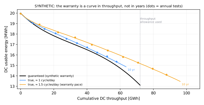
Two synthetic batteries, identical except for how hard they are used:
| Year | ≈ 1 cycle/day: throughput | headroom | ≈ 1.5 cycles/day: throughput | headroom |
|---|---|---|---|---|
| 1 | 7.3 GWh | +0.07 MWh | 11.4 GWh | +0.29 MWh |
| 3 | 21.1 GWh | +0.29 MWh | 32.9 GWh | +0.64 MWh |
| 5 | 34.0 GWh | +0.23 MWh | 52.5 GWh | +0.93 MWh |
| 7 | 46.1 GWh | +0.19 MWh | 70.8 GWh | +1.96 MWh |
| 9 | 57.8 GWh | +0.35 MWh | allowance used | warranty over |
Low use doesn't buy warranty headroom
The guarantee is indexed to throughput, but the battery also ages with time. Cycle a battery gently and its guaranteed energy stays high (little throughput), while calendar fade carries on regardless. The headroom of the battery used about once a day hovers between 0.1 and 0.35 MWh, around 1–2 %. The real battery's first-year test sat just as close: 20.10 MWh measured against 20.04 guaranteed. The battery used at the warranty's pace builds far more headroom. Then it uses up its allowance in year 8, and the warranty ends, whatever the date.
5 · Counting cycles: rainflow¶
A state-of-charge trace is not a neat series of full cycles. It's a big daily swing with regulation and FCAS wiggles on top. Rainflow counting (ASTM E1049) pairs each rise with the fall that closes it, like rain running down a pagoda roof. A small wiggle inside a big swing becomes one small cycle, and the big swing survives intact.
The algorithm keeps a stack of turning points. For each new point it compares the
latest range \(X\) with the previous range \(Y\). If \(X \ge Y\), then \(Y\) is a
closed cycle: count it and remove its two points. If \(Y\) includes the start of the
history, count it as a half cycle. The library's rainflow reproduces the ASTM
worked example and matches an independent implementation on 200 random histories
(see the tests).
Why bother? Because damage isn't linear in depth. With cycle damage \(\propto \text{DoD}^\beta\) and \(\beta \approx 1.25\), one 80 % cycle wears about 70 % more than eight 10 % cycles that move the same energy. A day of FCAS wiggles is cheap; a deep evening discharge is not.
6 · A model of fade¶
The synthetic battery uses \(k_\text{cal} \approx 0.96\) %/yr (0.08 %/month, the reference battery's calendar figure). The fade rate doubles for every 10 °C, and each string gets a slightly different frailty. That is the truth the estimators below try to recover.
7 · Tracking state of health: estimation is optimisation¶
Two kinds of measurement:
- Annual capacity test: precise (≈ 0.3 %) but rare. It goes stale for a year.
- Daily operational estimate: on days with a deep cycle, energy moved ÷ SOC change. It's frequent but noisy (≈ 2.5 %), and it reads low when cold and high when warm.
Fitting a straight line \(E = E_0 + sQ\) to all measurements, weighted by precision, is weighted least squares (T3). Doing it recursively, updating as each measurement arrives, is the Kalman filter. With state \(x = (E, s)\) and throughput increment \(\Delta Q\):
Each measurement carries its own \(\sigma_k\), so the gain automatically gives a test
about 70 times the weight of a daily estimate. With no process noise \(w_k\), the
filter returns exactly the least-squares line (a test checks this against
np.polyfit). A little process noise lets the slope drift, because fade isn't
really linear.
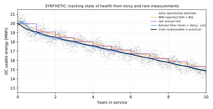
Over ten synthetic years, against the truth:
| Estimator | RMSE | Bias |
|---|---|---|
| Last annual test, held until the next | 0.35 MWh | +0.30 (stale, optimistic) |
| BMS SOH × BOL energy | 0.39 MWh | +0.29 (optimistic by design here) |
| 30-day median of daily estimates | 0.23 MWh | +0.03 |
| Kalman filter, tests + daily | 0.12 MWh | −0.02 |
The filter is three times as accurate as the last test. It costs nothing but arithmetic on data the plant already logs.
8 · When will it reach end of life?¶
Extrapolate the filtered trend to a threshold, here 80 % SOH, and sample the filter's posterior to get an interval.
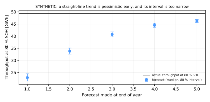
On the synthetic battery used about once a day, SOH actually reaches 80 % at 49.3 GWh, in year 7.4. The forecasts:
| Forecast made at end of year | Median | 80 % interval | Years left (forecast) | Years left (actual) |
|---|---|---|---|---|
| 1 | 22.9 GWh | 21.5–24.5 | 2.2 | 6.4 |
| 2 | 33.8 GWh | 32.6–35.1 | 2.7 | 5.4 |
| 3 | 40.7 GWh | 39.7–41.8 | 2.8 | 4.4 |
| 4 | 44.5 GWh | 43.7–45.3 | 2.4 | 3.4 |
| 5 | 46.2 GWh | 45.6–46.9 | 1.8 | 2.4 |
An interval is only as honest as its model
The straight-line model extrapolates today's slope. Early in life the slope still carries the fast formation fade, so early forecasts are pessimistic. The 80 % intervals are also too narrow: each one shrinks as data accumulate, yet the next year's forecast falls outside it. The filter knows how uncertain its parameters are. It doesn't know that its model is wrong. Report end-of-life forecasts with a model-error allowance, and re-fit them yearly.
9 · The price of a cycle¶
The unit error¶
The analytics guide computed
but 20.13 is the battery's usable energy in MWh, not its replacement cost in millions of dollars. Even with a real replacement cost, spreading the whole cost over the warranted throughput is wrong, because the battery still has ≈ 65 % of its capacity at the end. The defensible accounting cost charges each MWh discharged for the capacity it uses up:
The shadow price of a throughput budget¶
The warranty offers a better answer. Spread over the years it assumed, it allows a certain throughput per month. Put that budget into the Chapter 2/9 LP as a constraint:
LP duality gives the budget a shadow price \(\lambda^\star\): what one more MWh of allowance would earn this month. And the Lagrangian says something stronger:
has the same optimal value as the budgeted problem. So setting \(k_{deg} = \lambda^\star\) in the unconstrained LP makes the same decisions. The degradation cost to bid is the shadow price of the throughput budget.
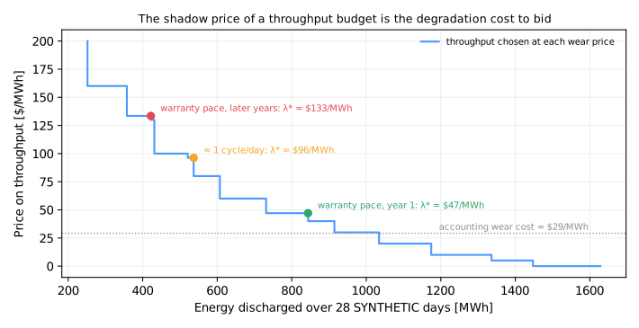
Over 28 synthetic days (the Chapter 9 market):
| Budget, as a yearly rate | Budget for 28 days | \(\lambda^\star\) | Revenue | vs no budget |
|---|---|---|---|---|
| No budget (\(k_{deg} = 0\)) | (1,628 MWh used) | $0 | $444,563 | — |
| Warranty pace, year 1: 11,000 MWh/yr | 844 MWh | $47/MWh | $430,176 | −3.2 % |
| ≈ 1 cycle/day: 7,000 MWh/yr | 537 MWh | $96/MWh | $409,479 | −7.9 % |
| Warranty pace, later years: 5,500 MWh/yr | 422 MWh | $133/MWh | $396,463 | −10.8 % |
Read it as a demand curve for cycling. The first few hundred MWh of throughput are worth a lot. Halving throughput from 1,628 to 844 MWh costs only 3 % of revenue, because the dropped cycles were barely profitable. Every \(\lambda^\star\) in the table exceeds the $29 accounting cost. When the budget binds, throughput is scarcer than the cells' wear, and the optimiser should bid the scarcity price.
At exactly \(\lambda^\star\) the answer ties
With \(k_{deg} = \lambda^\star\), the unconstrained LP is indifferent between throughput levels around the budget. The solver may return a different schedule with the same objective, revenue − \(\lambda^\star\) × throughput. That is T2's non-uniqueness in a new place, and the test suite checks the objective, not the schedule.
Solving a month one day at a time¶
The budget is the only constraint linking the days. Price it at \(\lambda\) and the month splits into independent daily LPs, each starting and ending at 50 % SOC. Total throughput falls as \(\lambda\) rises, so bisection finds the \(\lambda\) that meets the budget:
| Iteration | 1 | 2 | 3 | 4 | 5 | 6 | 7 | 8 | 9 | 10 |
|---|---|---|---|---|---|---|---|---|---|---|
| \(\lambda\) [$/MWh] | 0 | 1,000 | 500 | 250 | 125 | 62.5 | 93.8 | 109.4 | 101.6 | 105.5 |
| Throughput [MWh] | 1,633 | 7 | 12 | 115 | 435 | 760 | 592 | 509 | 555 | 536 |
At the ≈ 1 cycle/day budget it lands at λ = $105.5/MWh after ten rounds of 28 daily solves. The days could be solved in parallel. The Lagrangian dual value, \(\sum_d \max(\text{profit}_d) + \lambda B = \$403{,}909\), is an upper bound on any schedule within the budget that returns to 50 % SOC every day. The daily schedules earn $403,849, within $60 of it. It is not a bound on the month-long LP, which carries energy across midnight and earns $409,479. Decoupling the days was a restriction, and its cost shows up both as lost revenue and as a higher price, \(\lambda = \$105.5\) against the monolithic $96. This is the pattern behind decomposition at scale (Milestone 8): price the coupling constraint, solve the pieces separately, and adjust the price.
Why these techniques? Structure → method¶
| Property of the problem | Here | So |
|---|---|---|
| Wear depends on cycle depth, not only on energy moved | damage \(\propto \text{DoD}^{\beta}\), \(\beta \approx 1.25\), on a state-of-charge trace with small wiggles inside big swings | rainflow counting to turn the trace into cycles |
| State of health is hidden | two measurements of very different precision (annual test ≈ 0.3 %, daily estimate ≈ 2.5 %) of a slowly drifting quantity | a recursive estimator: the Kalman filter (weighted least squares, updated as data arrive) |
| Fade model | calendar, cycle and early-life terms with fixed parameters | simulate forward; extrapolate the filtered trend with a posterior interval |
| Throughput budget | one linear constraint added to the Chapter 2/9 LP | LP duality: its multiplier \(\lambda^\star\) is the price to bid |
| Coupling across days | the budget is the only constraint linking days | Lagrangian decomposition: price it, solve each day alone, adjust the price by bisection |
| Objective and constraints | linear in every dispatch variable | each daily problem is an LP that HiGHS solves in milliseconds |
Chosen. - Rainflow because fatigue damage is convex in depth. One 80 % cycle wears about 70 % more than eight 10 % cycles that move the same energy, so a count of megawatt-hours cannot see the difference. Rainflow pairs each rise with the fall that closes it. - The Kalman filter because the quantity of interest cannot be read from a meter. It combines a fade model with noisy tests, weights each by its own variance, and gives an uncertainty for the end-of-life forecast. With no process noise it reproduces the least-squares line exactly. - LP duality and the Lagrangian because the wear price should come out of the economics, not be assumed. Setting \(k_{deg} = \lambda^\star\) in the unconstrained LP reproduces the budgeted decisions. - Decomposition by day because it shows how a coupling constraint is priced and how the pieces become independent, which is the pattern at fleet scale.
Not chosen. - A flat cost per MWh from replacement cost. The $278/MWh in the analytics guide is a unit error, and even a correct flat cost ignores scarcity. The defensible accounting figure is about $29/MWh. The shadow prices are $47–133/MWh when a budget binds. - Equivalent full cycles (energy ÷ capacity). It treats shallow and deep cycling alike and understates the wear of deep discharges. - The last annual test, or the BMS state of health. The first goes stale for a year and the second is optimistic: RMSE 0.35 and 0.39 MWh against 0.12 MWh for the filter. - One month-long LP. At this size it is the better answer ($409,479 against $403,849 for daily decoupling) and needs no bisection. Decomposition is shown for scale, not because it wins here.
What the theory guarantees. - For an LP, strong duality gives a \(\lambda^\star\) equal to the slope of optimal revenue against the budget. At a kink it is a range, which is why the schedule ties. - Weak duality makes the Lagrangian value an upper bound on any schedule within the budget that is decoupled by day. - The filter is the exact posterior only if the model is linear and Gaussian. The chapter shows its 80 % intervals are too narrow because the model, not the parameters, is wrong.
References. - ASTM E1049-85 (2017) and Downing and Socie (1982), Rainflow counting: the definition and the compact algorithm. - Xu et al. (2018), Modeling of lithium-ion battery degradation: puts cycle depth into a cost an optimiser can use. - Schmalstieg et al. (2014), A holistic aging model: a published calendar-plus-cycle model. - Kalman (1960), A new approach to linear filtering: the recursive estimator.
All are in Further reading, Chapter 10. Duality is covered by Bertsimas and Tsitsiklis (1997) in Chapter 1's list. See also Choosing a technique.
10 · Implementation¶
import numpy as np

from energy_or.bess.cycle_price import price_of_throughput
from energy_or.bess.fcas import ALL_SERVICES
from energy_or.bess.lifecycle import WarrantyCurve, end_of_life, kalman_soh, rainflow
from energy_or.data.bess_life import bess_life

life = bess_life(years=10, efc_per_day=0.95)  # SYNTHETIC
z = life.op_estimate_mwh.copy()  # daily estimates, NaN on shallow days
sd = np.where(np.isfinite(z), 0.5, 1.0)
z[life.test_days], sd[life.test_days] = life.test_full_mwh, 0.06  # annual tests
kf = kalman_soh(life.throughput_mwh, z, sd, initial_energy_mwh=20.0)

warranty = WarrantyCurve()
headroom = kf.energy_mwh - warranty.energy_mwh(life.throughput_mwh)
eol = end_of_life(kf, threshold_mwh=16.0, throughput_per_year_mwh=7_000)
11 · Interpret¶
- Health: quote the filtered estimate with its band, not the BMS figure and not a year-old test.
- Warranty: track headroom continuously. A battery used gently has thin headroom, because calendar ageing isn't in a throughput-indexed curve. Expect next year's test to be close.
- End of life: a range, re-fitted every year, with model error acknowledged.
- Price of a cycle: about $29/MWh of wear at most. When a throughput budget binds, the right price is its shadow price, here $47–133/MWh. Never $316.
12 · Backtest¶
Re-run Chapter 9's backtest with \(k_{deg}\) set to the shadow price for the budget the owner wants to keep, and compare throughput and adjusted profit. The notebook does this on a short window. The reliable pattern is the one in the table above: halving throughput costs only a few per cent of revenue.
13 · Adding realism¶
- Weakest string. The plant's SOC limits act on the weakest string, so one weak string costs usable energy for all of them. Track string spread, and rebalance.
- Settlement structure. Many warranties compute each year's deficit as
guaranteed minus measured, averaged over the tests at the start and end of the year,
and settle the sum over five years. A surplus can offset a later deficit
(
warranty_deficit). - Delayed start. If commissioning slips, the BOL guarantee is re-based for
calendar fade on the idle cells (≈ 0.08 %/month,
WarrantyCurve.rebased). - RTE fade. Efficiency falls too, by ≈ 5 points over the warranty. That raises the break-even spread and lowers the value of every cycle.
- Augmentation. Adding strings to hold a contracted capacity is an investment timing problem, a dynamic program or MILP over years: Chapter 11.
14 · Exercises¶
Guided
Run rainflow on the trace 50 → 90 → 80 → 90 → 20 → 50 % by hand, then check it
in code. How many equivalent full cycles is it?
Engineering
Write a daily job that updates the Kalman filter from the day's counters and estimate, and raises an alert when the headroom falls below two standard deviations.
Market
The trader wants to keep the warranty's year-1 pace. Using the cycle-price curve, what \(k_{deg}\) should the optimiser use this month? What if FCAS prices halve?
Challenge
Show that the Lagrangian dual function \(g(\lambda) = \max_x [\,\text{revenue}(x) - \lambda(\text{throughput}(x) - B)]\) is convex and piecewise linear in \(\lambda\), and that throughput at \(\lambda\) is a subgradient. Replace bisection with a subgradient method and compare iterations.
Production challenge
The BMS SOH jumps 2 % after a firmware update, and one string's counter resets to zero. Design the data-quality checks that stop either from corrupting the filter.
15 · Production perspective¶
- SOH is a data product. It needs daily inputs (counters, deep-cycle estimates, temperature), annual tests, a filter, an alert and a version history.
- Measure what the contract measures. That means DC full-range energy at rated power, interpolated at the measured throughput. Keep the operating-window figure for trading, and never mix the two.
- Feed the price of a cycle back to dispatch. Recompute \(\lambda^\star\) monthly from the budget and the price outlook, and log it with every schedule.
- Treat end-of-life forecasts like any forecast: backtest them, and report their errors.
Run it yourself¶
| Artefact | Location |
|---|---|
| Warranty curve, rainflow, fade model, Kalman SOH, end of life | src/energy_or/bess/lifecycle.py |
| Price of a cycle (shadow price, Lagrangian by day) | src/energy_or/bess/cycle_price.py |
| Synthetic battery life | src/energy_or/data/bess_life.py |
| Tests | tests/test_bess_lifecycle.py |
| Notebook | notebooks/10_battery_life.ipynb |