2 · A battery and a day of prices: energy and FCAS
Foundation Intermediate Case B LP → MILP FCAS

In this chapter
- Model a battery as an LP with time coupling: what you do now changes what you can do later
- Write the state-of-charge (SOC) equation with charge and discharge losses, inside a 3–97 % operating envelope
- Read the dual of the SOC equation as the value of stored energy
- See why round-trip losses and degradation cost set a minimum price spread, and how a degradation cost cuts cycling from ~3 to ~1 cycle per day
- Meet the first constraint an LP cannot express, no simultaneous charge and discharge, and fix it with a binary variable (MILP)
- Co-optimise energy and eight FCAS markets: shared headroom, SOC reserved to back enabled services, and why FCAS can be most of a battery's revenue
1 · The real-world problem
A 10 MW / 20 MWh battery sits in the NEM. Over a typical day the regional price falls through the middle of the day, sometimes below zero, as rooftop and utility solar flood the region, then climbs steeply into the evening peak.
The obvious strategy is "buy low, sell high". But it's not obvious how much to buy, when exactly, and whether a $40/MWh spread is worth the wear on the cells. With 288 five-minute intervals in a day, there are far too many combinations to reason through by hand.
Arbitrage is only part of the story
For one operating NEM battery whose settlement data informed this chapter, FCAS earned roughly two-thirds of its 2023 market revenue, and energy arbitrage the rest. Sections 1–13 build the energy-only model, because every co-optimised model builds on it; Section 14 adds FCAS.
2 · The physical system
| Element | What limits it |
|---|---|
| Inverter | Charge and discharge power ≤ 10 MW |
| Cells | Usable energy 20 MWh. Operated between 3 % and 97 % SOC to protect the cells and keep headroom for control |
| Losses | Charging stores only \(\eta_c\) of the energy drawn; discharging delivers only \(\eta_d\) of the energy removed |
| Wear | Every MWh cycled consumes some of the battery's life |
Losses mean a round trip of 1 MWh in returns only \(\eta_c\eta_d\) MWh. With \(\eta_c = \eta_d = 0.92\) that is 84.6 %.
3 · The decision
For every 5-minute interval of the day, how many MW should the battery charge, and how many should it discharge?
Unlike Chapter 1, the intervals are not independent. Energy sold at 18:00 must have been bought earlier, and the battery can only hold so much.
4 · Decision variables
| Symbol | Meaning | Units |
|---|---|---|
| \(c_t\) | Charging power in interval \(t\) | MW |
| \(d_t\) | Discharging power in interval \(t\) | MW |
| \(SOC_t\) | Energy stored at the start of interval \(t\) | MWh |
\(SOC_t\) is a state variable. We don't choose it directly; the dynamics below set it from the \(c\) and \(d\) we choose. Including it as a variable keeps the model readable and gives us its dual for free.
| Parameter | Value |
|---|---|
| \(P_{max}\) | 10 MW |
| \(E_{max}\) | 20 MWh |
| SOC envelope | \(0.03E_{max} = 0.6\) MWh to \(0.97E_{max} = 19.4\) MWh |
| \(\eta_c,\ \eta_d\) | 0.92, 0.92 |
| \(\Delta t\) | 5 min = 1/12 h |
| \(RRP_t\) | Regional price for interval \(t\) [$/MWh] |
| \(k_{deg}\) | Degradation cost [$/MWh discharged], 0 to start with |
5 · Objective
Energy sold earns \(RRP_t \cdot d_t \Delta t\); energy bought costs \(RRP_t \cdot c_t \Delta t\). Over the day:
Units again
\(RRP\) is in $/MWh, \(d\) in MW, \(\Delta t\) in hours, so every term is in $. Forget the \(\Delta t\) and a 5-minute schedule earns twelve times too much.
6 · Constraints
| Constraint | Physical meaning |
|---|---|
| \(SOC_{t+1} = SOC_t + \eta_c c_t \Delta t - \dfrac{d_t \Delta t}{\eta_d}\) | Energy is conserved, minus losses |
| \(0.03E_{max} \le SOC_t \le 0.97E_{max}\) | Stay in the operating envelope |
| \(0 \le c_t \le P_{max},\ 0 \le d_t \le P_{max}\) | Inverter limit |
| \(SOC_0 = 0.5E_{max}\) | We start half full |
| \(SOC_T \ge SOC_0\) | We may not end the day emptier than we started |
The last constraint matters. Without it, the "optimal" plan is to sell the energy you started with, which looks like profit but is really just running down inventory. A terminal condition is how a one-day model avoids borrowing from tomorrow.
7 · Mathematical formulation
Why these techniques? Structure → method
| Property of the problem | Here | So |
|---|---|---|
| Objective | revenue \(RRP_t(d_t - c_t)\Delta t\) minus a linear wear term | linear: an LP |
| Variables | \(c_t, d_t, SOC_t\), all continuous | 865 variables for one day. The graphical method cannot be drawn; a simplex or interior-point solver is needed |
| Constraints | 288 equalities (the SOC equation) and bounds; \(SOC_T \ge SOC_0\) is a \(\ge\) row | the solver adds a slack for each \(\le\), a surplus for the \(\ge\) and, in a textbook simplex, an artificial variable for each equality (big-M or two-phase) to find a first corner. HiGHS does this internally |
| Time coupling | \(SOC_{t+1}\) depends on \(SOC_t\) | a chain of equalities: sparse, banded, easy for an LP, hard to reason about by hand |
| Simultaneous charge and discharge | not forbidden by any linear row | needs an on/off variable \(u_t\): a MILP, solved by branch and bound |
| Uncertainty | prices assumed known (perfect foresight) | a deterministic model; the cost of that assumption is measured in Chapter 9 |
| Size and speed | under 10 ms (LP), about 0.5 s a week (MILP) | exact methods are fast enough that heuristics are unnecessary |
Chosen. - An LP for the energy-only and FCAS models. Linear objective and linear dynamics fit exactly, the optimum is global, and the duals of the SOC equations are the value of stored energy used throughout the book. The FCAS joint-capacity rows are also linear, so co-optimising eight services adds variables, not a new technique. - A MILP only where the LP is wrong. The binary \(u_t\) with \(c_t \le P_{max}u_t\) and \(d_t \le P_{max}(1-u_t)\) uses the natural bound \(P_{max}\) as its big-M. No smaller constant is valid, so the relaxation is as tight as this formulation allows. - HiGHS through SciPy, with a tight relative gap when the LP and MILP must be compared to the cent.
Not chosen. - A threshold rule ("charge below \(x\), discharge above \(y\)"). It ignores the SOC coupling between intervals and the losses, gives no bound on how far it is from optimal, and has no shadow prices. - Dynamic programming on a discretised SOC. It handles non-convex wear easily, but it discretises the state, is slower as services are added, and yields no duals. It returns in Chapter 11, where the state is a battery's age and an LP is not available. - A MILP for everything. At positive prices the LP never charges and discharges together, so the binary only adds solve time and loses the duals. - Stochastic programming or MPC now. Both belong once a deterministic answer exists to be compared against; the perfect-foresight LP is also the upper bound used in backtests.
What the theory guarantees. An LP solved to optimality gives the global optimum, and strong duality gives the value of stored energy as a certificate (Bertsimas and Tsitsiklis, 1997). Dropping the integrality of \(u_t\) is a relaxation, so the LP profit is an upper bound on the MILP profit. Branch and bound (Land and Doig, 1960) stops with a proven gap to the best possible value, which is the optimality gap in the OptOps note.
References. - Conejo, Carrión and Morales (2010) and Morales et al. (2014): scheduling and offering models for storage and stochastic generation (Chapter 2). - Williams (2013), Model Building in Mathematical Programming: logical conditions such as "not both" as binary variables (same section). - Land and Doig (1960), branch and bound (Choosing a technique). - Bellman (1957), Dynamic Programming: the alternative not chosen here (same section). - Choosing a technique for how this fits the rest of the book.
It is still an LP: every term is a constant times a variable. For one day it has \(288 + 288 + 289 = 865\) variables and 288 equality constraints. HiGHS solves it in under 10 ms.
8 · Visualisation
Read the three panels together: price on top, dispatch in the middle (charging below the axis, discharging above), SOC at the bottom.
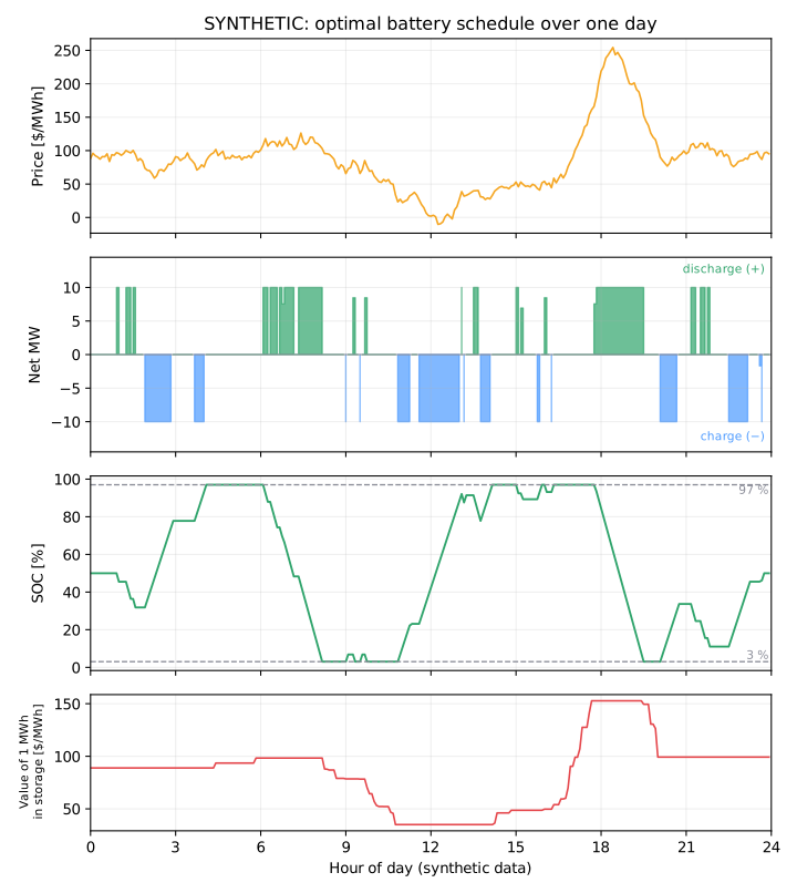
The optimiser does what an experienced trader would, but exactly:
- Charge in the overnight lull and through the midday solar trough.
- Hold when the spread to the next opportunity doesn't cover the losses.
- Discharge into the morning shoulder and the evening peak.
- It runs two cycles: full (97 %) by 04:00, empty (3 %) after the morning shoulder; full again by late afternoon, empty (3 %) by 19:30 after the evening peak. Both envelope limits bind, twice.
9 · Python implementation
from energy_or.bess import BatterySpec, optimise_arbitrage
from energy_or.data.synthetic import nem_price_days

prices = nem_price_days(1, seed=11).rrp_per_mwh  # SYNTHETIC, 288 intervals
battery = BatterySpec(
    power_mw=10,
    energy_mwh=20,
    soc_min_frac=0.03,
    soc_max_frac=0.97,
    eta_charge=0.92,
    eta_discharge=0.92,
)
result = optimise_arbitrage(prices, battery, interval_minutes=5)
optimise_arbitrage (src/energy_or/bess/arbitrage.py) builds the matrices
directly with scipy.sparse, because the model has thousands of variables. Variables
are laid out as \([c_0..c_{T-1},\ d_0..d_{T-1},\ SOC_0..SOC_T]\); each row of the
equality matrix is one SOC-dynamics equation.
10 · Solve
BESS SCHEDULE

  Battery           10 MW / 20 MWh, SOC 3%–97%, round trip 84.6%
  Horizon           288 × 5-min intervals
  Intervals         charge 71, hold 156, discharge 61
  Energy            bought 57.85 MWh, sold 48.96 MWh (2.60 equivalent full cycles)
  SOC               start 50.0%, end 50.0%, min 3.0%, max 97.0%

  Energy revenue    $3,999.58
  Degradation cost  $0.00
  Profit            $3,999.58

  Value of 1 MWh in storage: $35.01 – $152.77/MWh over the horizon
11 · Interpret
Bought 57.85 MWh, sold 48.96 MWh: where did 8.9 MWh go?
Into heat. With \(\eta_c\eta_d = 0.846\), every MWh bought returns 0.846 MWh, so the battery must earn its losses back through the price spread. Check: \(57.85 \times 0.846 = 48.96\). SOC starts and ends at 50 %, so the books balance exactly.
Losses set a minimum spread
Buying at \(p_{buy}\) and selling at \(p_{sell}\) is only worth it if
Buy at $100 and you must sell above $118. The test suite checks both sides of this line ($110 does not trade, $130 does).
The value of stored energy
The dual of each SOC equation answers: if one extra MWh appeared in the battery at this moment, how much more profit would the day make? Over this day it ranges from $35 to $153/MWh:
- It is low in the midday trough, where energy is plentiful and the battery is filling anyway.
- It is high before the evening peak, where an extra MWh would be sold at peak prices.
This is the battery equivalent of a hydro operator's water value, and it is how a real trading desk thinks: don't sell energy for less than it is worth in storage. Later chapters use it to turn an optimised schedule into bids.
Many cycles, small margins
With no wear cost the battery does 2.6 equivalent full cycles in a day. A lot of that is chasing small, noisy spreads, each just above the 18 % loss hurdle. On a spreadsheet those trades look free. On the cells they are not.
12 · Degradation: when is a spread worth the wear?
Calibrating \(k_{deg}\)
Measured state-of-health (SOH) data from an operating grid-scale battery fleet (72 racks, about 22 weeks, kept confidential and not published) shows capacity fading at roughly 2–2.5 % per year, with about 1 percentage point of spread between racks. Turning that into a $/MWh cost needs assumptions, shown here explicitly:
| Quantity | Value | Source |
|---|---|---|
| Capacity fade | ≈ 2.25 %/yr | Observed (fleet SOH data) |
| Share of fade due to cycling (vs calendar ageing) | ≈ 50 % | Assumed |
| Throughput | ≈ 1 cycle/day × 18.8 MWh ≈ 6,900 MWh/yr | Assumed |
| Value of 1 % of capacity | 20 MWh × $250k/MWh ÷ 20 % usable fade ≈ $250k | Assumed |
Treat $40/MWh as an order of magnitude, not a fact. The method is the point: measured fade + explicit assumptions → a cost the optimiser can trade against. Chapter 10 derives the number properly: as the shadow price of the warranty's throughput budget.
What it does to the schedule
Over a synthetic week:
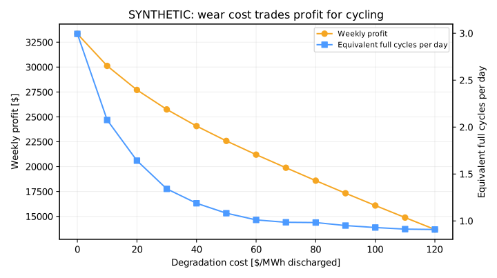
| \(k_{deg}\) [$/MWh] | Energy revenue | Profit after wear | Cycles/day |
|---|---|---|---|
| 0 | $33,340 | $33,340 | 2.99 |
| 20 | $32,026 | $27,703 | 1.64 |
| 40 | $30,328 | $24,073 | 1.19 |
| 60 | $29,185 | $21,202 | 1.01 |
| 80 | $28,938 | $18,590 | 0.98 |
At $40/MWh, energy revenue falls by only 9 %, but cycling falls by 60 %. Most of the dropped trades were barely profitable. The optimiser now keeps the big daily spread (solar trough → evening peak) and drops the noise. That is what the spec meant by "add degradation and show why the solution changes".
Perfect foresight
These numbers assume the whole week's prices are known in advance. Real revenue is lower. Measuring how much lower, honestly and without look-ahead bias, is the job of the backtesting framework (Chapter 9), and closing the gap is the job of forecasting and rolling-horizon control.
13 · Adding realism: the first non-linear rule
A real inverter cannot charge and discharge in the same instant. The LP has no rule against it, and normally doesn't need one, because doing both just burns energy.
At negative prices, burning energy pays. The battery is paid to import, so if it is nearly full, it can import more by charging and discharging at once, wasting the difference as heat. In a 12-hour test (6 h at −$50/MWh then 6 h at $30/MWh, starting 90 % full), the LP does exactly that in 6 intervals and reports a profit the physical battery cannot achieve.
The rule "\(c_t > 0 \Rightarrow d_t = 0\)" is not linear. It needs an on/off decision, a binary variable \(u_t \in \{0,1\}\):
When \(u_t = 1\) the battery may charge but not discharge; when \(u_t = 0\) the reverse. The model is now a mixed-integer linear program (MILP):
| LP | MILP | |
|---|---|---|
| Simultaneous intervals (negative-price test) | 6 | 0 |
| Profit | higher (unphysical) | lower (achievable) |
| Duals / value of storage | yes | no, MILPs have no simple duals |
| Solve time, one week | ~40 ms | ~0.5 s |
The LP is a relaxation of the MILP: it allows everything the MILP allows, and more. So its profit is always an upper bound. When prices are all positive, the two agree, and the test suite checks that too.
OptOps: the optimality gap
MILP solvers stop when the best solution found is provably within a small gap of the best possible. HiGHS's default is 0.01 %. On one test day that left the MILP $0.18 below the LP. The library asks for a tighter gap so the two can be compared to the cent. In production, the gap is a setting you choose and a metric you monitor, traded against solve time.
14 · Adding FCAS: energy and ancillary services together
The problem
So far the battery sells one thing: energy, in MWh, at the regional price. In the NEM it can also sell frequency control ancillary services (FCAS): megawatts of capability held in reserve, ready to push frequency back towards 50 Hz. FCAS is paid per MW enabled per hour, whether or not it is called on.
| Market family | What it does | Services modelled |
|---|---|---|
| Regulation | Continuously follows AEMO's AGC signal, correcting small imbalances | RAISEREG, LOWERREG |
| Contingency | Responds automatically after a large disturbance (e.g. a unit trip) | RAISE / LOWER 6SEC, 60SEC, 5MIN |
That makes eight markets. Very fast 1-second raise and lower services were added in October 2023; they are left out here for brevity, and adding them is an exercise.
A battery is very good at FCAS: it can swing from full charge to full discharge in well under a second. But energy and FCAS draw on the same two resources:
- Headroom (MW). A battery discharging 10 MW for energy has no room left to raise. One charging at 10 MW can raise a long way, by charging less and then discharging.
- Stored energy (MWh). Promising to raise for 10 minutes needs energy in the tank to back it. Promising to lower needs empty space to absorb it.
The question becomes: how should every MW and every MWh be split between energy and eight FCAS markets, interval by interval?
New decision variables
| Symbol | Meaning | Units |
|---|---|---|
| \(r_{k,t}\) | MW enabled for FCAS service \(k\) in interval \(t\) | MW |
| \(\pi_{k,t}\) | FCAS price for service \(k\) (a parameter) | $/MW/h |
New constraints
Headroom. For each raise contingency service \(k\):
and symmetrically for lower: \((c_t - d_t) + r_{\text{LOWERREG},t} + r_{k,t} \le P_{max}\).
Notice what is not written: the three raise contingency services are not summed. They act on successive timescales after the same disturbance (6 s, then 60 s, then 5 min), so the same headroom can back all three. This mirrors the structure of the NEM's FCAS joint capacity constraints: energy plus regulation plus each contingency service, one at a time. It is the reason a battery can earn several FCAS prices from one MW.
Energy backing. Enough SOC must be stored to sustain the enabled response:
applied at the start and end of every interval, with sustain times \(\tau\) in minutes:
| Service | \(\tau\) (teaching approximation) | Why |
|---|---|---|
| 6SEC | 1 min | Sustained until the 60SEC service takes over |
| 60SEC | 5 min | Sustained until the 5MIN service takes over |
| 5MIN | 10 min | Sustained until dispatch re-balances |
| REG | 5 min | One full interval of full-scale regulation |
Regulation uses energy. Regulation moves continuously, so a fraction \(u\) of the enabled MW (assumed 15 %) flows as energy. It changes SOC, is settled at the spot price, and wears the battery. Contingency events are rare and their energy is ignored here.
Formulation
subject to the Section 7 constraints (with regulation energy added to the SOC equation), plus headroom, energy backing and \(0 \le r_{k,t} \le P_{max}\). It is still an LP: one day is about 3,200 variables and 7,200 constraints, and solves in roughly 0.1 s.
from energy_or.bess import cooptimise_energy_fcas
from energy_or.data.synthetic import nem_fcas_prices, nem_price_days

prices = nem_price_days(1, seed=11).rrp_per_mwh
fcas = nem_fcas_prices(1, seed=11)  # SYNTHETIC, 8 services, $/MW/h
result = cooptimise_energy_fcas(prices, fcas)
print(result.explain())
Solve
BESS ENERGY + FCAS SCHEDULE

  Battery           10 MW / 20 MWh, SOC 3%–97%
  Horizon           288 × 5-min intervals
  Cycles            3.31 equivalent full cycles

  Energy revenue    $3,112.08
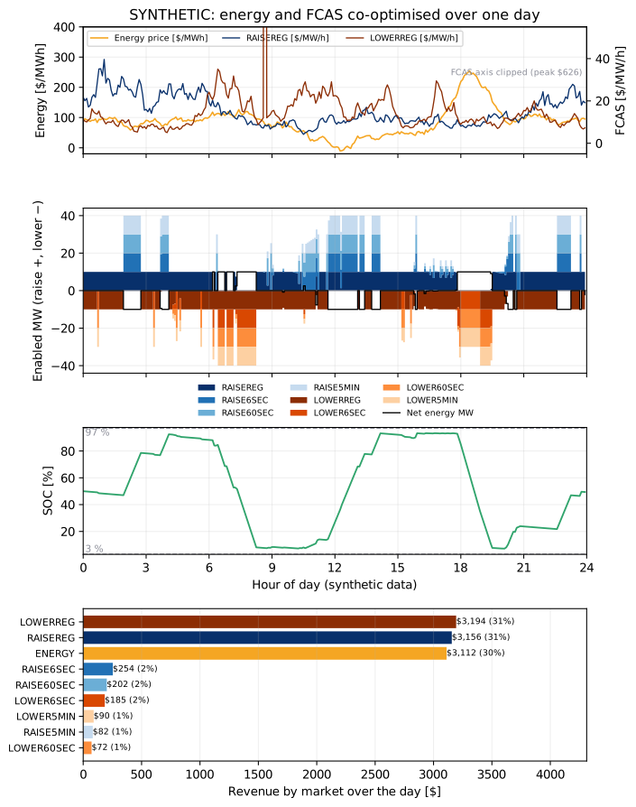
  RAISEREG          $   3,156.27   (avg  7.94 MW enabled)
  LOWERREG          $   3,193.77   (avg  7.38 MW enabled)
  RAISE6SEC         $     253.85   (avg  2.58 MW enabled)
  RAISE60SEC        $     201.99   (avg  2.53 MW enabled)
  RAISE5MIN         $      81.99   (avg  2.33 MW enabled)
  LOWER6SEC         $     184.53   (avg  1.68 MW enabled)
  LOWER60SEC        $      71.72   (avg  1.65 MW enabled)
  LOWER5MIN         $      89.57   (avg  1.59 MW enabled)
  Degradation cost  $0.00
  Profit            $10,345.78   (FCAS share 70%)
Interpret
The battery gives up energy revenue on purpose. Energy-only, it earned $4,000 on this day. Co-optimised, its energy revenue falls to $3,112, but total profit rises to $10,346. Every MW discharged for energy in the evening is a MW that cannot be enabled for raise. The optimiser trades a little arbitrage for a lot of FCAS.
Regulation dominates, and is not free. RAISEREG and LOWERREG earn more than 60 % of the day's revenue. They also push throughput up (3.31 cycles, versus 2.60 energy-only), because regulation energy passes through the cells. With a degradation cost, that wear is now priced against the regulation price.
SOC is kept away from both edges. Raise services need energy above the floor; lower services need room below the ceiling. The energy-only battery spends 39 % of the day within 5 points of an SOC limit; co-optimised, only 23 %. That is the value of being half full.
Headroom is always full. Because every FCAS service pays something, the raise headroom constraint binds in essentially every interval: any MW not used for energy is sold as capability. What changes through the day is who gets it. In the evening peak (17:30–19:30) the battery discharges 8.3 MW on average, and RAISE6SEC enablement collapses from a daily average of 2.6 MW to 0.2 MW. That is the trade-off the co-optimisation exists to make.
Over a synthetic week
With degradation at $40/MWh (Section 12):
| Energy only | Energy + FCAS | |
|---|---|---|
| Weekly profit | $24,073 | $69,241 |
| FCAS share of revenue | — | 69 % |
| Equivalent full cycles per day | 1.19 | 2.24 |
The 69 % FCAS share sits close to the roughly two-thirds seen in the 2023 settlement data of the operating battery mentioned in Section 1. The synthetic FCAS prices were calibrated to be in that range; the model was not tuned to hit it.
What this co-optimisation leaves out
- Price-taking. FCAS markets are shallow. A 10 MW battery can move FCAS prices, and every new battery in the region competes for the same revenue. Real FCAS revenue has fallen as storage has grown. A price-taker model overstates it.
- Perfect foresight of both energy and FCAS prices.
- FCAS trapezia, enablement limits and bids. NEMDE enables FCAS from offers, not from a private optimiser. This model decides what a battery would want; bidding to get it is Part V.
- Contingency deployment energy, and regulation cost recovery and performance-based payments.
- The sustain times and the 15 % regulation utilisation are teaching assumptions.
15 · Exercises
Guided
Predict the profit for prices [0, 0, 100, 100] (60-min intervals), lossless,
starting and ending at 3 %. Why does the battery charge 10 MW then only 8.8 MW?
(Answer: $1,880.)
Engineering
Add a ramp-rate limit \(|net_t - net_{t-1}| \le R\). Write it as two linear constraints. How does a tight ramp limit change the evening discharge?
Market
Raise \(k_{deg}\) until the battery stops trading on an ordinary day but still
trades on a spike day (spike_probability=1.0). What does that say about
reserving cycles for spikes?
Challenge
Make the terminal SOC a decision with a value: replace \(SOC_T \ge SOC_0\) with a reward \(v_{end} \cdot SOC_T\) in the objective. How should \(v_{end}\) relate to the stored-energy duals you saw?
Production challenge
The schedule is re-solved every 5 minutes with fresh price forecasts. The battery's measured SOC disagrees with the model's SOC by 0.8 MWh. Which one do you trust, what do you log, and what do you alert on?
16 · Production perspective
- Rolling horizon. In operation the model is re-solved every interval on a forecast horizon; only the first interval's decision is executed (Milestone 9).
- Telemetry first. \(SOC_0\) must come from the battery's own measurement, not from the model's previous answer. Drift between the two is an incident (see the incident labs).
- Safety envelope. 3–97 % is the commercial envelope inside the OEM's hard limits; the controller must clamp setpoints whatever the optimiser says.
- Explain. Log the schedule, binding SOC limits, the value of stored energy, and the
SolveReport(status, solve time, size, MILP gap). - FCAS enablement is not the same as FCAS dispatch. The optimiser says what the battery would like to be enabled for; NEMDE decides from bids. Monitor enabled vs offered per service, and the SOC reserve actually held.
- Market depth. Track FCAS prices against the region's storage fleet: revenue assumptions built on last year's FCAS prices age quickly.
Run it yourself
| Artefact | Location |
|---|---|
| Energy model | src/energy_or/bess/arbitrage.py |
| Energy + FCAS model | src/energy_or/bess/fcas.py |
| Synthetic prices | src/energy_or/data/synthetic.py → nem_price_days, nem_fcas_prices |
| Tests | tests/test_bess_arbitrage.py, tests/test_bess_fcas.py |
| Animations | animations/bess/arbitrage.py, animations/bess/fcas.py |
| Notebook | notebooks/02_bess_arbitrage.ipynb |