15 · Committing a battery before the prices are known
Intermediate Advanced Case B Two-stage stochastic programming · Benders · SAA · CVaR

In this chapter
- A 10 MW / 20 MWh battery must decide, for a whole season and before any day's
prices are known:
- how many MW to reserve for a network-support contract;
- how many MW of $300 caps to sell.
Every day it then trades whatever is left - Formulate the decision as a two-stage stochastic programme: decide now, recourse later - Measure two values, \(\text{EEV} \le \text{RP} \le \text{WS}\): - the value of the stochastic solution: what planning on the average day costs; - the expected value of perfect information - Solve the problem three ways: - one big LP (the extensive form) - Benders (L-shaped) decomposition - sample-average approximation with statistical bounds - Make it risk averse with CVaR (Chapters 13–14) - Backtest with a recourse that cannot see the day's prices, and find that the textbook model, which assumes hindsight, reserves too little
Chapter 9 traded a battery day by day. Chapter 11 planned its life year by year. This chapter sits between them: commitments made once, before the uncertainty, that constrain every day's trading after it. That shape, decide now and adapt later, is the defining structure of stochastic programming, and recognising it is half the work.
1 · The real-world problem
A battery owner is offered two contracts for the coming season:
- Network support. The transmission network wants fast reserve: keep \(x\) MW of discharge headroom, and enough energy to run it for 30 minutes, available at all times. The network uses it to protect a corridor after a fault. It pays $600 per MW per day. Some large batteries run public schemes of this kind. The terms here are illustrative.
- Caps. A retailer will buy \(y\) MW of $300 caps: it pays a premium of $244 per MW per day, and the battery owner pays \((p - 300)^+\) per MWh in every half-hour the price exceeds $300. The board requires caps to be physically backed: \(x + y \le 10\) MW.
Whatever is not committed is traded in the spot market every day. Both decisions must be made now, for the whole season.
2 · The physical and market system
- Battery: 10 MW / 20 MWh, state of charge 3–97 %, 92 % efficiency each way, a $5/MWh wear cost on discharge (Case B; Chapters 2, 10 and 11). Each day starts at 50 % and must end at least there.
- Prices: 1,000 synthetic half-hourly days (
energy_or.data.battery_days): - an ordinary duck curve on most days;
- a short evening spike on 12.5 % of days;
- a scarcity event of 2–5 hours at $400–$4,000 on 2.8 % of days.
Each day also has the day-ahead forecast an operator would have had, which never contains the events. - The cap market's view: the retailer priced the cap on a market where scarcity happens on 1 % of days. Our scenarios say about 3 %. That disagreement is the commercial heart of the problem.
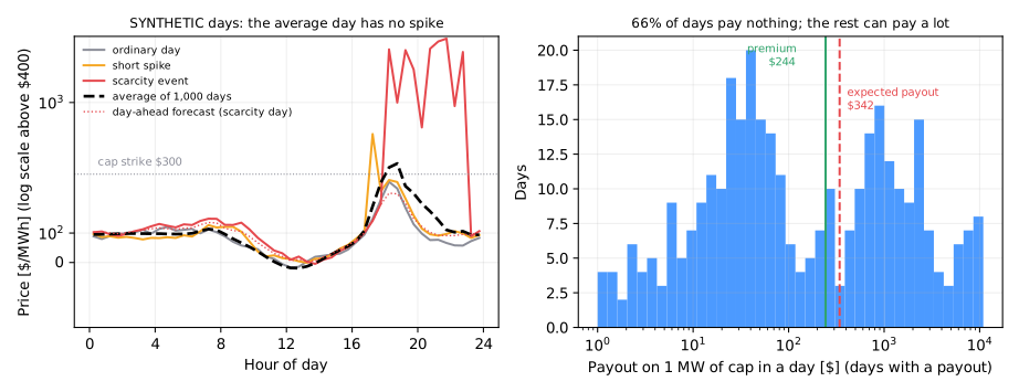
Two facts stand out in the figure: - 66 % of days pay nothing on a cap, and a few pay over $10,000 per MW; - the average of 1,000 days barely crosses $300. Its cap payout is $29 per MW-day, against a true expected payout of $342.
3 · The decision
| Stage | When | Decision | Knows |
|---|---|---|---|
| First (here and now) | before the season | \(x\) MW reserved, \(y\) MW of caps | the distribution of days, not which days will come |
| Second (recourse) | each day | charge and discharge in each half-hour | that day's prices |
The first-stage decision is the same for every scenario: it cannot depend on a day it has not seen. This is non-anticipativity, and it is what makes the problem stochastic rather than 1,000 separate deterministic ones.
4 · Variables
- First stage: \(x \in [0, 10]\) MW, \(y \ge 0\) MW.
- Second stage, for each scenario day \(s\) and half-hour \(t\): charge \(c_{st}\), discharge \(d_{st}\) [MW] and state of charge \(e_{st}\) [MWh]: 3 × 48 = 144 variables per day, 144,002 in total for 1,000 days.
5 · Objective
Expected daily profit:
where \(Q_s(x)\) is the best trading profit on day \(s\) given the reservation:
Notice that \(y\) enters only through the expected payout. A cap is a financial contract, and the battery's dispatch does not change what it pays out.
6 · Constraints
For each day \(s\) and half-hour \(t\), with \(\Delta t = 0.5\) h:
- Energy balance: \(e_{st} = e_{s,t-1} + \eta_c c_{st}\Delta t - d_{st}\Delta t / \eta_d\).
- Headroom for the reserve: \(d_{st} \le P - x\) (equivalently \(d_{st} + x \le P\)).
- Energy for the reserve: \(e_{st} \ge e_{\min} + x \cdot 0.5\,\text{h} / \eta_d\).
- Envelope: \(e_{\min} \le e_{st} \le e_{\max}\), \(0 \le c_{st}, d_{st} \le P\), \(e_{s,48} \ge e_{s,0}\).
- Backing: \(x + y \le P\).
The first-stage variable \(x\) appears in every day's constraints. That is the coupling, and it is why the days cannot be solved independently.
7 · Formulation
Why these techniques? Structure → method
| Property of the problem | Here | So |
|---|---|---|
| Decisions in two stages | \(x, y\) before the season; dispatch after each day is revealed | Two-stage stochastic programme with recourse (Dantzig, 1955) |
| Uncertainty | a distribution of days, known only through samples, with rare high-impact events | scenarios (a sample average), not a single forecast |
| Objective and constraints | linear in every variable, given the scenarios | each scenario's recourse is an LP, and the whole problem is one LP |
| Recourse value \(Q_s(x)\) | concave and piecewise linear in \(x\) (an LP's value as its right-hand side changes) | supporting hyperplanes (cuts) from the duals describe it exactly: Benders / L-shaped (Benders, 1962; Van Slyke and Wets, 1969) |
| Size | 1,000 days × 144 variables, linked only by \(x\) | the extensive form is large but block-structured; decomposition exploits the blocks |
| Sample size vs truth | the optimum is fitted to the sample | SAA bounds to say how good the answer really is (Mak, Morton and Wood, 1999) |
| Decision-maker | a board with a risk appetite | mean–CVaR of daily profit, which stays an LP (Rockafellar and Uryasev, 2000) |
Chosen. - The extensive form writes all scenarios and one copy of \((x, y)\) in a single LP. Non-anticipativity is automatic, because there is only one \(x\). HiGHS solves it to proven optimality. - The L-shaped method solves the same problem without ever building it. A small master problem in \((x, y, \theta)\) proposes a commitment. The 1,000 daily LPs, which are independent once \(x\) is fixed, report their value and the duals of the reserve rows. Each round adds one cut \(\theta \le Q(x_k) + g_k (x - x_k)\). - SAA answers a question the other two cannot: with 30, 100 or 365 days, how far is the sample's answer from the true optimum? - CVaR adds risk with \(S + 1\) extra variables and keeps everything linear.
Not chosen. - The expected-value (EV) problem, which replaces the scenarios with the average day. It is solved here only to show what it costs. Averaging destroys exactly the rare events that decide the cap's value (Birge, 1982). - A deterministic model with a safety margin, such as "reserve 1 MW less than the EV plan". The margin has no basis and no measure of value. The stochastic programme computes the trade-off instead. - A multi-stage stochastic programme, which re-decides every half-hour as information arrives. That is closer to reality, but scenario trees grow exponentially. The two-stage model plus a realistic backtest (section 12) gives most of the insight. - Robust optimisation, which plans for the worst case in a set. Its answer would be "never sell caps". The distribution is reasonably known, so averaging over it is more appropriate than guarding against its extreme. Chapter 16 takes the opposite case, where the distribution cannot be trusted and a guarantee is required.
What the theory guarantees. - The extensive form and the L-shaped method reach the same global optimum: the problem is an LP, and the cuts are exact because \(Q\) is concave. - \(\text{EEV} \le \text{RP} \le \text{WS}\) always holds (Birge, 1982), so the VSS and EVPI are never negative. - The SAA optimum is biased upwards. Evaluating its decision on fresh scenarios is unbiased. Together they bracket the true optimum (Mak, Morton and Wood, 1999; Kleywegt, Shapiro and Homem-de-Mello, 2002).
References. Further reading, Chapter 15, plus Birge and Louveaux (2011) for the textbook treatment and Choosing a technique for how this fits the rest of the book.
The extensive form
The L-shaped method
Master problem after \(K\) cuts:
Here \(Q(x_k)\) is the average daily trading profit at the trial \(x_k\). The slope \(g_k\) comes from the recourse duals: each MW reserved tightens the 48 headroom rows by 1 MW and the 48 energy rows by \(0.5/\eta_d\) MWh, so \(g_k = -\sum_t(\lambda^{\text{head}}_{t} + 0.5\,\lambda^{\text{energy}}_{t}/\eta_d)\) averaged over days.
8 · Visualisation
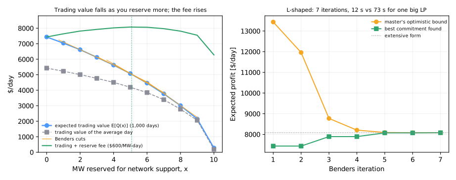
Left: reserving each MW costs trading value. - Reserving 5 MW costs about $2,350 a day; 10 MW costs almost everything. - The orange tangents are the Benders cuts, and the green curve adds the fee. Its peak is the optimum. - The average day undervalues trading by about $2,000 a day at every reservation level (grey). Averaging smooths away the spikes a battery earns most from.
Right: the master problem's optimistic bound falls and the best commitment found rises until they meet, after 7 iterations.
9 · Implementation
from energy_or.data.battery_days import battery_days
from energy_or.risk.two_stage import (
    evaluate_commitment,
    expected_value_solution,
    l_shaped,
    market_terms,
    saa_bounds,
    simulate_realistic,
    solve_two_stage,
    wait_and_see,
)

terms = market_terms()  # fee $600/MW-day; cap premium priced on the market's view
days = battery_days(1_000, seed=31)  # SYNTHETIC
rp = solve_two_stage(days, terms)  # extensive form
ev = expected_value_solution(days, terms)  # plan on the average day
eev = evaluate_commitment(days, ev.reserve_mw, ev.cap_mw, terms)
ws = wait_and_see(days, terms)  # hindsight, day by day
ls = l_shaped(days, terms)  # Benders
cautious = solve_two_stage(days, terms, tail_weight=0.5)  # mean–CVaR
10 · Solve: three answers to "what should we commit?"
| Method | Reserve \(x\) [MW] | Caps \(y\) [MW] | Expected profit [$/day] | Solve |
|---|---|---|---|---|
| Plan on the average day (EV) | 5.90 | 4.10 | believes $8,309; gets $7,665 (EEV) | single day |
| Stochastic programme (RP), extensive form | 5.08 | 0 | $8,081 | 74 s |
| Stochastic programme, L-shaped | 5.09 | 0 | $8,081 | 12 s, 7 iterations |
| Perfect hindsight (WS), each day its own commitment | varies | varies | $10,188 | 1,000 small LPs |
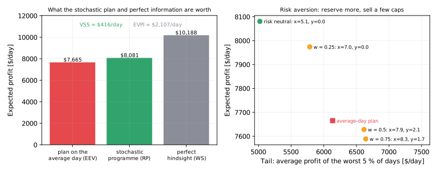
- VSS = RP − EEV = $416 a day, about $152k a year. The average-day plan sells 4.1 MW of caps, because on the average day caps almost never pay. Across the real distribution they pay $342 a MW-day on average, for a premium of $244. The stochastic programme sells no caps: it sees the scarcity days.
- EVPI = WS − RP = $2,107 a day. This is the most any forecast could be worth to these commitments. Hindsight would reserve all 10 MW on dull days and nothing on volatile ones.
- Decomposition pays. The L-shaped method finds the same commitment six times faster, because each round solves 1,000 small independent LPs instead of one LP with 144,002 variables. The advantage grows with the number of scenarios.
11 · Interpret
- The structure of the answer: reserve where the fee beats the trading value lost (about 5 MW, where trading's marginal value per MW falls below $600). Sell caps only if the premium beats the expected payout: here it does not.
- The disagreement is the trade. The retailer's premium is fair on its 1 % view of scarcity, and too cheap on our 3 % view. If our view is right, selling caps transfers money to the retailer. If theirs is right, we are leaving $244 a MW-day on the table. The model makes this explicit. Exercise 3 asks at what scarcity probability the decision flips.
- Risk aversion (right panel): with weight \(w\) on the average of the worst 5 % of days, the battery reserves more and sells a few caps.
| Weight on the tail | \(x\) | \(y\) | Mean [$/day] | Worst-5 % average [$/day] |
|---|---|---|---|---|
| 0 (risk neutral) | 5.08 | 0 | 8,081 | 5,020 |
| 0.25 | 6.97 | 0 | 7,974 | 5,785 |
| 0.5 | 7.85 | 2.15 | 7,628 | 6,617 |
| 0.75 | 8.27 | 1.73 | 7,589 | 6,644 |
This surprises at first: a risk-averse battery sells caps it expects to lose money on. The reason is that a battery's worst days are not scarcity days. Those are its best days, with the cap payout netted against spike revenue. Its worst days are dull days with a flat price and nothing to trade. Fee and premium are earned on every day, including the dull ones, so for a battery they are the hedge.
12 · Backtest: a recourse you can actually run
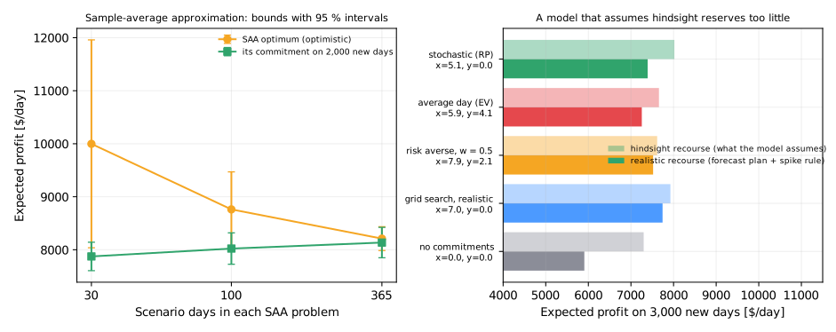
The stochastic programme assumes that each day's dispatch is chosen with that day's prices known. A real battery commits its plan from a forecast and reacts as the day unfolds. Each commitment is therefore re-run on 3,000 new days, with a recourse that: - plans the day with the LP on the day-ahead forecast (reserve respected); - then discharges as hard as headroom and energy allow whenever the realised price exceeds $300, the cap-cover rule.
A grid search over \((x, y)\) in 1 MW steps, scored with this realistic recourse on 1,000 separate days, is the simulation-based answer.
| Commitment | \(x\), \(y\) | Hindsight recourse [$/day] | Realistic recourse [$/day] | Realistic worst-5 % [$/day] |
|---|---|---|---|---|
| Stochastic programme (RP) | 5.1, 0 | 8,020 | 7,392 | 4,867 |
| Plan on the average day (EV) | 5.9, 4.1 | 7,657 | 7,255 | 2,194 |
| Risk averse, \(w = 0.5\) | 7.9, 2.1 | 7,616 | 7,520 | 6,481 |
| Grid search, realistic recourse | 7, 0 | 7,926 | 7,742 | 5,651 |
| No commitments | 0, 0 | 7,298 | 5,906 | 2,422 |
What the backtest teaches:
- The model is only as good as its recourse. With hindsight dispatch, the stochastic programme's commitment is best ($8,020). With realistic dispatch it earns $628 a day less, because it reserved too little: it priced trading flexibility as if the battery always knew when the spike was coming. The commitment chosen against the realistic recourse reserves 7 MW and earns $350 a day more (about $128k a year).
- The average-day plan has the worst bad days ($2,194): sold caps meet scarcity events the realistic battery cannot fully cover.
- The two-stage model still earns its keep. It identifies the structure of the answer (moderate reserve, no caps at this premium) and the VSS, and on hindsight dispatch it is exact. The fix is to close the gap between modelled and real recourse: a capture factor, a forecast-based recourse inside the model, or a multi-stage formulation.
How many scenarios? (left panel). The SAA optimum is optimistic: - with 30 days it promises $9,998 ± 1,961 a day, but its commitment earns $7,874 ± 268 on 2,000 new days; - with 365 days the gap closes to $75 (within the confidence intervals); - the recommended reserve swings by ± 2.8 MW between 30-day samples and by ± 0.6 MW at 365 days.
Rare events need many scenarios: a 3 % event appears about once in a 30-day sample.
13 · Adding realism
- Multi-stage. Decide the season's commitment now, then re-decide each day's plan as forecasts update. That needs a scenario tree or stochastic dual dynamic programming.
- Reserve activation. When the network triggers the reserve, the battery discharges, and must then recharge. Model activations as a random event with a recovery requirement.
- Seasonality and correlation. Scarcity clusters in winter evenings and in multi-day weather events. Sample whole weeks, not independent days.
- FCAS co-optimisation (Chapter 2) inside the recourse: reserved MW may still earn some contingency FCAS, depending on the network contract.
- Degradation. Reserved capacity cycles less. Credit it with the wear cost saved (Chapters 10–11).
14 · Exercises
Guided
Re-solve with the reserve fee at $400, $800 and $1,000 per MW-day and plot \(x\) against the fee. Explain the shape with the left panel of the L-shaped figure.
Engineering
The L-shaped method solves all 1,000 days in one block LP per iteration. Parallelise the days across processes and time it. At what number of scenarios does decomposition beat the extensive form by ten times?
Market
At what market view of scarcity probability does market_terms price the cap
fairly against our scenarios? Above it, the stochastic programme sells caps. Find
the switch.
Challenge
Prove that \(Q_s(x)\) is concave in \(x\), and that the L-shaped cuts are valid upper bounds. Start from LP duality, with \(x\) appearing only in the right-hand side.
Production challenge
Specify the seasonal commitment review: inputs, the scenario library and how it is refreshed, SAA bounds reported with each recommendation, and the realistic backtest that must pass before the board signs.
15 · Production perspective
- Report the bounds, not just the answer. Every recommendation comes with its SAA gap and the spread of the decision across samples.
- Validate the recourse model against what the trading system really achieves (Chapter 9's capture ratio). A model that assumes hindsight will over-commit to flexibility.
- OptOps for decomposition: log iterations, bound gap, cut count and time per subproblem batch, and alert when the gap stops closing.
- Commitments are governance decisions. The optimiser proposes, the board decides, and the contract's physical requirements (reserve, backing) go into the dispatch system as hard constraints, never as preferences.
Further reading
- Dantzig (1955): the first two-stage model under uncertainty.
- Birge (1982): the value of the stochastic solution and the bound ordering.
- Benders (1962) and Van Slyke and Wets (1969): decomposition with cuts from duals.
- Mak, Morton and Wood (1999) and Kleywegt, Shapiro and Homem-de-Mello (2002): how good is an SAA solution.
- Birge and Louveaux (2011): the textbook.
- Conejo, Carrión and Morales (2010): stochastic programming for electricity market participants.
Full citations with DOIs are in Further reading.
Run it yourself
| Artefact | Location |
|---|---|
| Extensive form, EV, WS, L-shaped, SAA, realistic recourse, grid search | src/energy_or/risk/two_stage.py |
| Synthetic price days with forecasts | src/energy_or/data/battery_days.py |
| Tests | tests/test_two_stage.py |
| Notebook | notebooks/15_committing_before_the_prices_are_known.ipynb |