4 · Choosing a maintenance window
Intermediate Part IX Cases D · E · G Enumeration → MILP

In this chapter
- Turn "when should we do the gearbox exchange?" into decision variables, hard constraints and an objective
- Put a value on downtime: forecast generation × value per MWh, hour by hour
- Handle the crane's wind limit with a weather-forecast ensemble: a window is not "safe", it is safe with some probability
- Return ranked windows with reasons, not a single unexplained answer
- Keep opportunity loss (planned on forecasts) apart from realised loss (measured on what happened), and backtest the planner over 40 synthetic weeks
- Schedule several jobs that share one crew: the first MILP of Part IX
1 · The real-world problem
A site manager has a job to place in the coming week:
Gearbox exchange, 24 hours of turbine outage. The first 7 hours are a crane lift that is only allowed in daylight with hub-height wind at or below 10 m/s. Technicians may not work at all above 18 m/s. Earliest Monday, latest Sunday.
Every hour the turbine is down costs the generation it would have made, valued at the spot price plus certificates. Wind and prices are forecasts. Which window should they book?
This is Case E (crane plus weather) and the core of Case G (the seven-day site-manager planner). Chapter 3 decided whether to replace a gearbox; this chapter decides when.
2 · The physical system
| Element | Constraint it imposes |
|---|---|
| Crane | Lift wind ≤ 10 m/s for 7 continuous hours, in daylight |
| Technicians | No work above the access limit (18 m/s) at any point in the job |
| Turbine | Produces nothing for the whole 24 h job |
| Weather | Known only as a forecast, increasingly uncertain with lead time |
| Market | Each MWh not produced is worth price + LGC (illustratively $35/MWh) |
The crane's wind limit is a hard safety constraint, not a cost. The optimiser never trades it against money. It only decides among windows that satisfy it.
3 · The decision
At which hour should the job start?
With hourly resolution over a week, there are 168 candidate start hours.
4 · Variables and data
| Symbol | Meaning | Units |
|---|---|---|
| \(t\) | Start hour of the job (the decision) | h |
| \(D\) | Job duration (24) | h |
| \(L\) | Crane hours at the start of the job (7) | h |
| \(W_s(\tau)\) | Forecast hub wind in hour \(\tau\), scenario \(s\) | m/s |
| \(P_s(\tau)\) | Forecast turbine output in hour \(\tau\) | MW |
| \(V(\tau)\) | Forecast value of one MWh: price + LGC | $/MWh |
The forecast is an ensemble of \(S = 40\) scenarios, synthetic here, whose spread grows from under 1 m/s at hour 0 to about 3 m/s six days ahead.
5 · Objective
The opportunity cost of starting at \(t\) in scenario \(s\) is the value of generation forgone:
and we minimise its expectation \(\bar C(t) = \frac{1}{S}\sum_s C_s(t)\), while reporting the P10–P90 spread so the manager can see the risk.
Computing this for every start is one cumulative sum: \(C(t) = Q(t + D) - Q(t)\) with \(Q(k) = \sum_{\tau < k} P(\tau)V(\tau)\). All 168 windows cost about as much to evaluate as one.
6 · Constraints
A start \(t\) is feasible only if:
| Constraint | Expression |
|---|---|
| Within allowed dates | \(t \ge t_{earliest}\), \(t + D \le t_{latest}\) |
| Lift in daylight | hours \(t, \dots, t + L - 1\) all in 07:00–17:59 |
| Crane-safe with confidence | \(\Pr_s\!\big[\max_{\tau \in [t, t+L)} W_s(\tau) \le 10\big] \ge 0.8\) |
| Access-safe with confidence | \(\Pr_s\!\big[\max_{\tau \in [t, t+D)} W_s(\tau) \le 18\big] \ge 0.8\) |
The crane condition is a chance constraint: it must hold in at least 80 % of forecast scenarios. The confidence level is a management choice, and Section 11 shows what it costs.
7 · Formulation
Why these techniques? Structure → method
| Property of the problem | Here | So |
|---|---|---|
| Decision, one job | one start hour, 168 candidates | one integer variable with a short list: enumerate. No graphical method or simplex is involved |
| Objective | expected generation forgone: a sum of forecast output × value | linear in the data; one cumulative sum prices every window |
| Safety limits | wind ≤ 10 m/s for 7 h, ≤ 18 m/s for 24 h | hard feasibility filters on each start, never traded against money |
| Uncertainty | 40 forecast scenarios of wind | a chance constraint on the ensemble: safe in at least 80 % of scenarios |
| Decision, many jobs | binaries \(x_{j,t}\): 6 jobs × 168 starts = 1,008 | MILP. Enumerating \(168^6\) combinations is out of reach |
| Constraint types (MILP) | \(\sum_t x_{j,t} = 1\) (equality), \(\sum x \le K\) (crews) | a solver adds an artificial variable for each equality, a slack for each \(\le\); big-M or two-phase finds the first corner of the relaxation |
| Size and speed | single job under a millisecond; crew MILP in seconds | exact methods are fast enough, so no heuristic |
Chosen. - Exhaustive enumeration for one job. The feasible set \(\mathcal{F}\) has at most 168 members, so checking all of them is an exact algorithm. It is also the most explainable one: every rejected start has a stated reason (daylight, dates, crane wind). - A chance constraint on the ensemble rather than on a single forecast. A window is safe with some probability, and the 80 % level is a management setting whose price the chapter shows (a 100 % level roughly triples the cost). - A time-indexed MILP for several jobs sharing a crew. The binary \(x_{j,t}\) ("job \(j\) starts at hour \(t\)") makes the crew limit a plain linear row, and HiGHS solves it by branch and bound. With one job it must return the enumeration's answer, which the tests check.
Not chosen. - A MILP for a single job. It would return the same answer more slowly and say less about why other starts lost. - A Gaussian formula for the chance constraint. The quantity is the maximum wind over 7 hours, which is not normal. The ensemble gives its distribution directly. - Robust optimisation (worst case of all scenarios). That is the 100 % row of the table in Section 11. It moves the job to a costlier day to avoid a 2 % risk, and the safety limit is not an optimisation variable anyway. - Placing jobs one at a time, each in its own best window. It can stack two jobs on one crew. The coupling between jobs is exactly what the MILP carries.
What the theory guarantees. Enumeration returns the global optimum over the feasible starts, and the MILP is proven optimal to a stated gap. The chance constraint holds for the ensemble, not for the real weather. How many scenarios make that carry over to the real weather is the subject of the scenario approach (Calafiore and Campi, 2006), which is stated for convex problems, so treat it as guidance for this discrete choice. A 40-member ensemble gives coarse probabilities.
References. - Charnes and Cooper (1959), chance-constrained programming; Prékopa (1995), probabilistic constraints; Calafiore and Campi (2006), the scenario approach; Gneiting and Raftery (2007), proper scores for probabilistic forecasts (Chapter 4). - Land and Doig (1960), branch and bound, and Dantzig (1963), slack and artificial variables (Choosing a technique). - Wolsey (2021), Integer Programming: why a time-indexed formulation is useful (Chapter 5). - Choosing a technique for how structure decides the method across the book.
For a single job, \(\mathcal{F}\) has at most 168 members, so evaluating every one is an exact optimisation algorithm, and the most explainable one possible: it can say why each rejected start was rejected. Reaching for a MILP solver here would add nothing. Section 13 shows where one becomes necessary.
8 · Visualisation
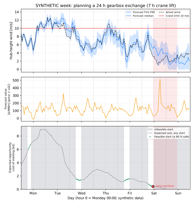
Read the panels from top to bottom: where the forecast wind dips below the crane limit in daylight, a lift is possible; where generation and value are low, the outage is cheap; the best window is where both happen together.
9 · Python implementation
from energy_or.data.forecast import maintenance_week
from energy_or.maintenance import MaintenanceJob, rank_windows

week = maintenance_week(seed=21)  # SYNTHETIC, hour 0 = Monday 00:00
job = MaintenanceJob(
    "Gearbox exchange WTG-07", duration_h=24, crane_hours=7, crane_wind_limit_ms=10.0
)
plan = rank_windows(
    job, week.wind_forecast_ms, week.value_forecast, week.hour_of_day, min_confidence=0.8
)
print(plan.explain())
rank_windows (src/energy_or/maintenance/window.py) computes every start's cost
with the cumulative-sum trick and the rolling maxima of wind with
sliding_window_view, then filters and ranks.
10 · Solve
RECOMMENDATION

Job:                Gearbox exchange WTG-07 (24 h, 7 h crane lift ≤ 10 m/s)
Maintenance window: Sat 11:00 – Sun 11:00

Primary drivers:
  • Forecast generation forgone 3.3 MWh (mean wind 3.4 m/s)
  • Value of that generation $126/MWh
  • Crane-safe in 98% of forecast scenarios

Binding constraints (starts rejected):
  • outside allowed dates: 23
  • lift outside daylight: 115
  • crane wind > 10 m/s (confidence < 80%): 12

Estimated opportunity cost: $422 (P10 $52 – P90 $770)

Alternatives:
  • Sat 10:00 – Sun 10:00: +$25, crane-safe 98%
  • Sat 09:00 – Sun 09:00: +$88, crane-safe 98%
This is the recommendation format the book's explainability rule asks for: what was chosen, why, which constraints bound, the estimated cost with its spread, and the next-best alternatives with their cost difference.
11 · Interpret
Daylight is the tightest constraint. 115 of 168 starts are rejected because the 7-hour lift would run into the night. Only 18 starts survive all constraints, in four clusters (Mon, Wed, Fri and Sat mornings).
Expected opportunity cost ranges from about $140 to $9,000 across starts that fit the horizon. The best window costs $422: a calm Saturday, forecast at 3.4 m/s, when the turbine would barely turn. The value per MWh in that window ($126/MWh) is not low. It is the volume that is low. Timing maintenance is mostly about wind, not price, for a wind farm; for a battery or a solar farm the balance differs.
The confidence level has a price. Demanding certainty changes the answer:
| Required crane-safe confidence | Feasible starts | Best start | Expected cost |
|---|---|---|---|
| 50 % | 20 | Sat 11:00 | $422 |
| 80 % | 18 | Sat 11:00 | $422 |
| 100 % | 4 | Fri 07:00 | $1,299 |
Insisting that every forecast scenario is safe moves the job to Friday and roughly triples its expected cost. That is not an argument for accepting more lifting risk, which is a safety decision made by people, not optimisers. It is an argument for making the trade-off visible: the 2 % of scenarios that rule out Saturday cost $877 of expected generation to avoid. A planner can also hold Saturday as the plan and Friday as the fall-back.
Opportunity loss is not realised loss. The plan is made on forecasts. What it actually cost is known only afterwards:
| Start | Expected (forecast) | Realised (what happened) |
|---|---|---|
| Sat 11:00 (planned) | $422 | $5 |
| Mon 07:00 (first feasible) | — | $6,473 |
The realised loss on Saturday turned out lower than forecast; on another week it might be higher. One week proves nothing. That is what backtests are for.
12 · Backtest: 40 synthetic weeks
For each of 40 synthetic weeks, plan on that week's forecast, then evaluate on that week's "actual" weather and prices. Three policies:
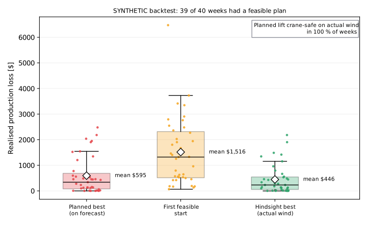
| Policy | Mean realised loss per job |
|---|---|
| Optimised on the forecast | $595 |
| First feasible window ("do it as soon as we can") | $1,516 |
| Perfect hindsight (an unreachable lower bound) | $446 |
- In 39 of 40 weeks a feasible window existed; in one week, none did. That is a genuine answer ("no safe window this week") that the planner must report, not hide.
- Every planned lift turned out crane-safe on the actual wind.
- The optimiser closes about 85 % of the gap between "as soon as possible" and perfect hindsight. The remaining gap is the value of a better forecast.
Synthetic backtest
The weather, prices and forecast errors are synthetic, and the "actuals" are drawn from the same model as the forecasts. A real backtest uses archived forecasts and archived outcomes, with only information available at planning time (Part XIX).
13 · Adding realism: several jobs, one crew
Real weeks have several jobs competing for one crane and one crew. Placing them one at a time, each in its own best window, can put two jobs on top of each other. Now the decisions interact, and enumeration no longer scales:
\(x_{j,t} = 1\) means job \(j\) starts at hour \(t\). This is a mixed-integer linear program; the crew constraint couples the jobs.
from energy_or.maintenance import schedule_jobs

schedule = schedule_jobs(jobs, [expected_costs_of(job) for job in jobs], crews=1)
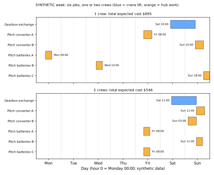
The test suite checks the obvious properties: for a single job the MILP returns exactly the enumeration's answer, and with one crew no two jobs overlap. Cranes, spares, travel and skills are added in Milestone 5, and this MILP is where they go.
14 · Exercises
Guided
Lower the crane limit to 8 m/s. How many starts survive, and what happens to the best window's cost?
Engineering
Real lifts need calm wind at the start (lift out) and the end (lift in) of a gearbox exchange. Change the feasibility check so both the first and the last 4 hours must be crane-safe.
Market
Give the turbine a PPA that pays a fixed $80/MWh regardless of spot, and a merchant neighbour on spot + LGC. Do the two rank windows differently? Why?
Challenge
Replace the chance constraint with a two-stage plan: book Saturday, but if on Friday the updated forecast puts the lift's safety below 80 %, switch to the best remaining window at a rebooking cost. Evaluate on the 40-week backtest.
Production challenge
The weather forecast arrives four times a day. Design how the planner re-runs, when it is allowed to change a booked window, and what it must log so that a rebooking can be explained to the crane contractor.
15 · Production perspective
- Inputs. Ensemble hub-height wind forecasts (not just the median), price forecasts, the turbine's power curve, and the job's safety limits from the method statement. Validate them: a missing forecast hour must not silently become "calm".
- Safety first. Wind limits come from the crane's and the procedure's documentation and are never optimised. The confidence level is set by the site, logged, and shown on every recommendation.
- Re-plan, don't drift. Re-run on every forecast update, but change a booked window only when the gain beats the cost of rebooking, and record why.
- Measure. Log forecast opportunity cost and realised loss for every job. Their difference, over months, tells you how much a better forecast would be worth.
Run it yourself
| Artefact | Location |
|---|---|
| Window optimiser + MILP | src/energy_or/maintenance/window.py |
| Synthetic forecast week | src/energy_or/data/forecast.py |
| Tests | tests/test_maintenance_window.py |
| Animation | animations/maintenance/crane_weather.py |
| Notebook | notebooks/04_maintenance_window.ipynb |