5 · A replacement campaign: crews, a crane and spares
Intermediate Advanced Part IX–XII Case C Time-indexed MILP

In this chapter
- Put reliability (Chapter 3), maintenance windows (Chapter 4), logistics and inventory into one optimisation model
- Build a time-indexed MILP: one binary per job per day
- Price waiting: lost generation for stopped turbines, expected failure cost for at-risk ones
- Model a crane properly: mobilisation + day rate + weather, so the optimiser bundles lifts into campaigns
- Treat spares as a cumulative inventory with deliveries and an expedite option
- Price the horizon boundary, or the model will defer work just to make its own cost look smaller
- Explain a MILP without shadow prices: what-if re-solves
1 · The real-world problem
Of the 28 turbines on a farm, 26 need work in the next six weeks:
| Turbines | Situation | Job | Needs |
|---|---|---|---|
| 2 | Stopped: pitch converter failed | Pitch converter module, 1 day | Electrical crew, pitch converter |
| 1 | Stopped: gearbox failed | Gearbox exchange, 4 days | Mechanical crew, crane (1 day), gearbox |
| 1 | Stopped: converter / fuse fault | Converter module, 1 day | Electrical crew, converter |
| 6 | At risk: gearbox debris alarms | Preventive gearbox exchange, 4 days | Mechanical crew, crane, gearbox |
| 16 | At risk: pitch batteries at end of life | Battery set replacement, 1 day | Electrical crew, battery set |
The mix follows the event-log patterns of Chapter 3: the pitch system causes most of the lost energy, stopped turbines wait days for parts, and gearbox exchanges are rare but need a crane. An end-of-life pitch battery set has a 0.4 % chance each day of failing its brake test and stopping the turbine until it is replaced.
Resources are limited: two mechanical crews and one electrical crew; one crane that the contractor can supply from day 5, at $120k per mobilisation plus $25k per day on site, lifting only on days whose daylight wind stays under its limit; three gearboxes in stock with two more arriving on day 21 (more can be expedited in 10 days at a $45k premium); no pitch converters in stock, two arriving on day 10 (or expedited in 4 days for $12k each); one converter module; and six battery sets with ten more arriving on day 14.
Which turbine should be repaired when, by whom, with which crane visit and which spare?
This is flagship Case C. All numbers are synthetic and illustrative.
2 · The physical system
Three resources, each with its own logic:
- Crews are a capacity: at most two mechanical jobs in progress on any day.
- The crane is a campaign: expensive to bring, expensive to keep, useless on windy days. Lifts should be bunched into one visit, but a visit kept open for weeks costs a fortune.
- Spares are an inventory: a gearbox used on day 5 is not available on day 15. Deliveries add stock; expediting buys stock early at a premium.
And two kinds of turbine:
- A stopped turbine loses its whole output every day it waits.
- An at-risk turbine still runs (perhaps derated), but every day it waits it might fail, causing secondary damage and stopping it.
3 · The decision
For each of the 26 jobs: which day to start, or defer it beyond the six-week horizon. Also: which days the crane is on site, and how many spares to expedite.
4 · Variables
| Symbol | Meaning | Type |
|---|---|---|
| \(x_{j,d}\) | Job \(j\) starts on day \(d\) | binary |
| \(u_j\) | Job \(j\) is deferred beyond the horizon | binary |
| \(k_d\) | Crane on site on day \(d\) | binary |
| \(m_d\) | Crane mobilised (arrives) on day \(d\) | binary |
| \(q_p\) | Spares of type \(p\) expedited | integer |
With 26 jobs over 42 days that is 1,206 variables: small for HiGHS, far too many combinations for a spreadsheet.
5 · Objective: put all the economics into start costs
The cleanest trick in time-indexed scheduling is to precompute, for every job and every possible start day, what starting then would cost. Then the constraints only have to describe resources.
Waiting cost per day \(w_j(\tau)\), with \(G(\tau)V(\tau)\) the value of one turbine's forecast generation that day:
where \(S_j(\tau) = (1 - p_j)^\tau\) is the chance an at-risk turbine is still running, \(\delta_j\) its derate, \(p_j\) its daily failure probability and \(F_j\) the extra cost of a failure (secondary damage, expediting). This is Chapter 3's reliability model turned into dollars per day.
Start cost: everything waited before the start, plus the outage during the job:
Starts that cannot work (the job would run past the horizon, or needs the crane on an unworkable or unavailable day) get \(c_{j,d} = \infty\) and are fixed to zero.
The objective:
6 · Constraints
| Constraint | Expression |
|---|---|
| Each job once, or deferred | \(\sum_d x_{j,d} + u_j = 1\) |
| Crews per skill per day | \(\sum_{j \in s}\ \sum_{d' \in (d - D_j,\, d]} x_{j,d'} \le K_s\) |
| Crane capacity, only when on site | \(\sum_{j \in crane}\ \sum_{d' \in (d - L_j,\, d]} x_{j,d'} \le \ell \, k_d\) |
| Count mobilisations | \(k_d - k_{d-1} \le m_d\) |
| Spares: cumulative use ≤ stock | \(\sum_{j \in p}\ \sum_{d' \le d} x_{j,d'} \le S_p(d) + q_p\,[d \ge \lambda_p]\) |
The spares constraint is the elegant one: cumulative starts up to day \(d\) cannot exceed cumulative availability up to day \(d\), including scheduled deliveries \(S_p(d)\) and expedited units once their lead time \(\lambda_p\) has passed.
Pricing the horizon boundary
A job deferred past day 42 still has to be done. If deferring costs only "waiting until day 42", the model will happily push expensive crane work past the horizon, where it becomes someone else's problem. The deferral cost therefore includes a further two weeks of waiting and the crane cost the job will still need later (here $65k: a share of a future mobilisation plus a crane day):
Section 11 shows what happens without it.
7 · Formulation, in code
Why these techniques? Structure → method
| Property of the problem | Here | So |
|---|---|---|
| Objective | start costs \(c_{j,d}\) precomputed, plus crane, expedite and deferral costs | linear in the variables, so the model is a linear programme with integrality |
| Variables | binaries \(x_{j,d}, u_j, k_d, m_d\) and integers \(q_p\): 1,206 for 26 jobs × 42 days | 26 × 42 choices cannot be enumerated or drawn. A MILP solver is needed, because a start day, a crane visit or an expedite is all-or-nothing |
| Constraint types | equalities (\(\sum_d x_{j,d} + u_j = 1\)), \(\le\) rows (crews, crane, spares), a linking row \(k_d - k_{d-1} \le m_d\) | in the LP relaxation each \(\le\) gets a slack variable and each equality an artificial variable, as in T0; HiGHS handles this internally |
| Time coupling | a job occupies a crew for \(D_j\) days; spares are a running stock | time-indexed binaries turn both into plain sums over days |
| Resources | crews and crane are capacities; spares are inventory | cumulative rows: starts up to day \(d\) ≤ stock up to day \(d\) |
| Uncertainty | failure risk enters as a daily probability; weather as workable days | expected costs in a deterministic model; Chapter 4's ensembles can replace the workable-day input |
| Size and speed | 362 constraints; a few seconds with a proven 0 % gap | exact solution is practical; heuristics are not needed |
Chosen. - A time-indexed MILP. "Job \(j\) starts on day \(d\)" is one binary, and every economic effect (waiting, outage, risk) is folded into its cost beforehand. The constraints then only describe resources, which keeps them short and linear. - Branch and bound with LP relaxations (HiGHS). The solver bounds the best possible cost at every step, so the answer comes with a proven gap, not just a plan. - A greedy baseline. It is a fair human rule and always feasible, so the 25 % saving is a real comparison and not a straw man. - What-if re-solves to price constraints, because a MILP has no useful duals.
Not chosen. - Big-M sequencing formulations, where binaries say which job comes before which. They use fewer variables but have weak relaxations, so branch and bound struggles; time-indexed models tend to give tighter bounds (Wolsey, 2021). - Constraint programming (CP-SAT). A strong alternative for scheduling with calendars and sequencing, and a natural next step if setup times and skills are added. Here the objective is linear cost with inventory, and the MILP gives a bound directly. - Dynamic programming over jobs. The state would carry crew use, the crane's status and every spare stock at once, which grows too fast to be practical. - Metaheuristics (genetic algorithms, annealing). They give no proof of how far from optimal they are, and at 1,206 variables an exact method finishes in seconds. - Greedy alone. It defers two gearbox exchanges and pays $120k more for crane time. Local rules cannot see that bunching lifts and buying parts early beat starting early.
What the theory guarantees. Branch and bound (Land and Doig, 1960) terminates with a solution and a lower bound; when the gap is zero the plan is optimal, as in Section 10. The LP relaxation is a lower bound on the MILP cost, and the tighter the formulation, the smaller the gap to close (Wolsey, 2021). Integer programmes do not have shadow prices in general, so the marginal values of a resource come from re-solving, not from duals.
References. - Wolsey (2021), Integer Programming, 2nd edition: formulation strength and time-indexed models (Chapter 5). - Land and Doig (1960), branch and bound; Dantzig (1963), slack and artificial variables in the relaxation; Charnes (1952), the big-M method (Choosing a technique). - Postek et al. (2025), Hands-On Mathematical Optimization with Python: worked scheduling models in Python (T1). - Choosing a technique for how structure decides the method across the book.
from energy_or.data.campaign import component_campaign
from energy_or.maintenance import optimise_campaign, greedy_campaign

problem = component_campaign()  # SYNTHETIC: 26 jobs, 42 days
plan = optimise_campaign(problem)  # time-indexed MILP, HiGHS
baseline = greedy_campaign(problem)  # worst-first, as early as possible
print(plan.explain())
optimise_campaign (src/energy_or/maintenance/campaign.py) builds each constraint
family as a sparse block and hands the lot to HiGHS through scipy.optimize.milp.
8 · Visualisation
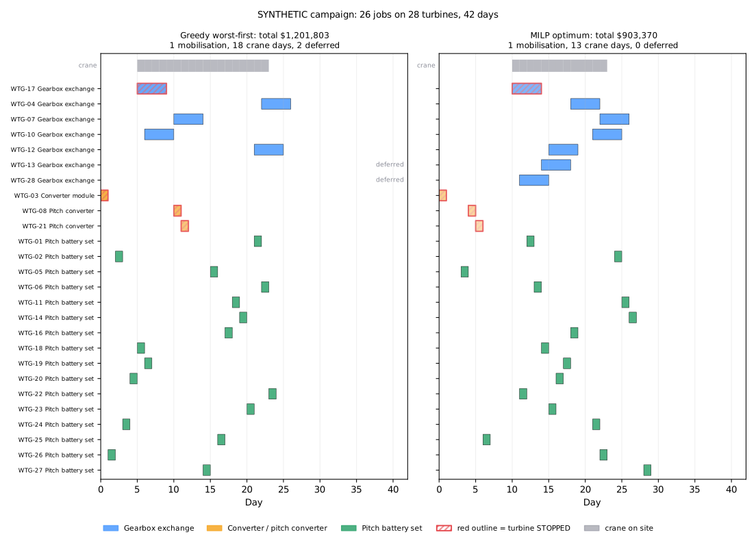
9 · The baseline: worst first, as early as possible
A sensible human rule: fix stopped turbines first, then the riskiest; start each job
on the earliest day its crew, spare and crane allow; keep the crane on site from the
first lift to the last. That rule is implemented as greedy_campaign, and it is a
fair benchmark: every plan it produces is feasible in the MILP.
10 · Solve
| Greedy worst-first | MILP | |
|---|---|---|
| Lost production and failure risk | $366,905 | $344,370 |
| Crane | $570,000 (18 days) | $445,000 (13 days) |
| Expedited spares | $0 | $114,000 (2 gearboxes, 2 pitch converters) |
| Deferred jobs (penalty) | $264,898 (2 gearbox exchanges) | $0 |
| Total | $1,201,803 | $903,370 |
The MILP is 25 % cheaper. HiGHS proves optimality (gap 0 %) in a few seconds on 1,206 variables and 362 constraints.
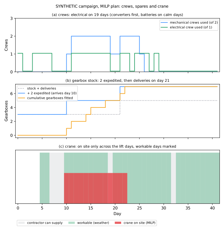
11 · Interpret
Buy the parts, bunch the crane, use the calm days
The greedy plan does the obvious things in the obvious order and still costs $300k more. The MILP makes three choices a site manager might not:
- It expedites both pitch converters ($24k) so the two stopped turbines restart on days 4 and 5 instead of waiting for the day-10 delivery. Each stopped turbine loses about $3,000 a day, so six days of waiting would cost more than the premium. This is Chapter 3's finding, that most lost energy is time spent waiting for parts, turned into a decision.
- It expedites two gearboxes ($90k) and times the crane to their arrival. The crane arrives on day 10, when the expedited gearboxes do, and stays 13 days to do all seven exchanges in one campaign. Greedy brings the crane on day 5, keeps it 18 days, and still defers two exchanges for lack of gearboxes.
- It replaces pitch batteries on calm days. A battery job stops the turbine for a day, while waiting another day risks only a 0.4 % chance of a failure. So the MILP puts the sixteen battery swaps on days worth, on average, a third of a typical day's generation ($1,000 against $3,060).
Why does the stopped gearbox turbine wait until day 10?
The crane is available from day 5, and the stopped gearbox turbine loses about $3,000 a day. Yet the MILP starts it on day 10. The alternatives explain why:
- Start it on day 5 and keep the crane: five more crane days before the next gearboxes arrive, about $125k.
- Start it on day 5 with a separate crane visit: a second mobilisation costs at least $120k, before its crane days.
- Wait: the turbine loses about $28k of generation over days 5–9, a windy spell.
Waiting is cheapest. It is a decision a site manager might question, so the plan must be able to explain it. And it is a decision that depends on the inputs: if that turbine were worth several times as much, or a crane mobilisation much less, the answer would change.
Explaining a MILP: what-if re-solves
An LP's duals price every constraint (Chapter 1). A MILP's do not exist in a useful form. The practical substitute is to change one input and re-solve:
from energy_or.maintenance import value_of_change

saving, new_plan = value_of_change(problem, crews={"mechanical": 3, "electrical": 1})
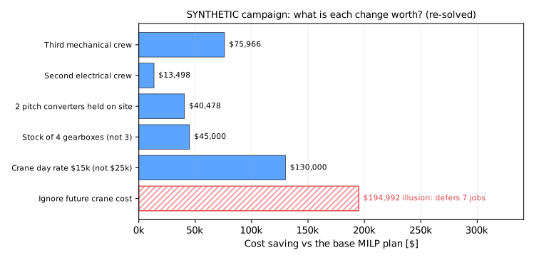
| What if… | Saving over the campaign | What changes |
|---|---|---|
| The crane day rate were $15k, not $25k | $130,000 | Same plan, cheaper crane |
| A third mechanical crew | $75,966 | Crane campaign shortened from 13 to 9 days |
| One more gearbox in stock | $45,000 | Exactly the expedite premium it avoids |
| Two pitch converters held on site | $40,478 | No expediting; both repaired on days 0 and 1 |
| A second electrical crew | $13,498 | Battery swaps done in pairs on the calmest days |
| Deferral ignored future crane cost | $194,992 | An illusion: all 7 gearbox exchanges pushed past the horizon |
Read the rows as business cases. Holding two pitch converters on site is worth about $40k on this campaign alone, before counting the next failure. A second electrical crew is worth little here: the battery swaps are mostly waiting for calm days, not for a crew. The last row is a warning: a model that doesn't price its horizon boundary reports a lower cost by doing less work. Always ask what an optimiser pushed outside its window.
12 · Backtest
A campaign plan is made on forecasts of wind, prices and failure risk, and executed over weeks while all three change. A credible backtest re-plans every few days (rolling horizon) using only information available at the time, executes the first days of each plan, and compares the realised cost with the greedy rule under the same realised weather and failures. That needs the backtesting framework (Milestone 7) and the rolling-horizon machinery (Milestone 9); this chapter's model is the engine they will call.
13 · Adding realism
- Travel and set-up. Moving the crane between turbines takes time, and crews travel. Add set-up days between consecutive crane jobs (a sequencing problem, Part X).
- Skills and fatigue. Crews with different competencies, shift limits and rest days (Part XII).
- Multi-site spares. Gearboxes held in a regional warehouse shared by several farms (Case F, Part XI).
- Weather uncertainty. Crane-workable days are forecasts; use Chapter 4's ensembles and re-plan.
- Network constraints. If several turbines sit behind a constrained connection, their outages cost less when the constraint would have curtailed them anyway (Chapter 1).
14 · Exercises
Guided
Make the at-risk gearboxes much riskier: 1.2 %/day and $250k secondary damage. Do the stopped turbines still go first? Explain the result using waiting costs.
Engineering
Add a second crane (lifts_per_day=2) with the same rates. How many crane days and
mobilisations does the new plan use, and is it worth it?
Market
Halve value_per_mwh (a low-price season). Which decisions change, and which stay
the same?
Challenge
Add a one-day crane relocation between consecutive lifts on different turbines. How does the formulation change? (Hint: the crane constraint becomes about pairs of jobs.)
Production challenge
The solve takes 4 s here and might take hours on a 100-turbine portfolio. Set
time_limit_s and mip_rel_gap, and decide what the planning service should do
with a feasible-but-not-proven-optimal answer. What do you log?
15 · Production perspective
- Inputs are the hard part. Failure probabilities come from condition monitoring and reliability models (Chapter 3), workable days from weather ensembles (Chapter 4), stock from the warehouse system, crews from the roster. Each needs validation and an owner.
- OptOps. Record status, solve time and MIP gap for every solve; alert when the gap or solve time drifts. A time-limited solve with a good incumbent is usable; silently using an infeasible one is not.
- Explain every plan. Publish the cost breakdown, the binding resources and a short list of what-ifs with every recommended schedule. Planners trust what they can interrogate.
- Re-plan without churn. Re-solve when forecasts or failures change, but penalise moving jobs that crews, crane and contractors have already been told about.
Run it yourself
| Artefact | Location |
|---|---|
| Campaign MILP, greedy baseline, what-ifs | src/energy_or/maintenance/campaign.py |
| Synthetic Case C | src/energy_or/data/campaign.py |
| Tests | tests/test_campaign.py |
| Animation | animations/maintenance/campaign.py |
| Notebook | notebooks/05_campaign_milp.ipynb |