13 · How bad can a year get? Measuring portfolio risk¶

Foundation Intermediate Case L Monte Carlo · VaR · CVaR · Shapley · backtesting

In this chapter

Turn "next year's revenue" from one number into a distribution, by simulating 2,000 years of the fictional Lantern Bay portfolio
Learn the vocabulary of risk on a real question:
- P50, P90, P99 (the energy industry's numbers)
- VaR and CVaR (the finance industry's)
- why one of them can make diversification look harmful
Find which assets and which drivers cause the bad years:
- Euler contributions split the bad years between the six assets
- a Shapley split shares them between weather, fuel, outages and certificates
Ask how sure we are: sampling error in a risk number, and how many years it takes to prove a risk model wrong

Every earlier chapter optimised against one forecast, or against a set of scenarios whose spread we did not look at closely. This chapter is about that spread. It needs no new optimiser, only one LP at the end. What it needs is a habit: before you optimise, ask what the range of outcomes is, what drives it, and how much you trust the answer. Chapter 14 then uses these measures as objectives and constraints.

Risk vocabulary used in this chapter

Term	Meaning here
Scenario	One possible year: weather, prices, outages and certificate price, settled through every contract
Distribution	All scenarios together, each with its probability (here equal)
P50 / P90 / P99	Revenue met or beaten in 50 / 90 / 99 % of years. P90 is the 10th percentile
Loss	How far revenue falls below a reference: here below the expected (mean) revenue
VaR95 (value at risk)	The loss exceeded in only 5 % of years: "how bad is a 1-in-20 year?"
CVaR95 (conditional VaR, expected shortfall)	The average loss in those worst 5 % of years: "when it is bad, how bad on average?"
Tail	The worst $1-\alpha$ of years (5 % for $\alpha = 0.95$)
Coherent	A risk measure that behaves sensibly: in particular, combining two portfolios never adds risk (subadditive)
Risk driver	A source of uncertainty that can be switched on or off in the model

1 · The real-world problem¶

The board of Lantern Bay Renewables is setting next year's budget. The CFO asks four questions that every asset owner hears:

What revenue should we budget? (The P50.)
What can we promise our lenders we will at least make? Lenders size debt on a P90 or P99 year, as in Chapter 7.
In a bad year, how bad, and is it bad because of the wind, the price, a broken transformer or the certificate market?
Which asset is the riskiest, and should we sell it, contract it or hedge it?

A single forecast cannot answer any of them. A distribution can.

2 · The physical and market system¶

Six fictional assets in four regions (three wind farms, a solar farm and two solar + battery hybrids), each with the illustrative contract described on the portfolio page. Revenue in a year is the sum of:

merchant energy: generation × regional price × loss factor;
contract flows: CfD difference payments, the as-produced PPAs' strike on their share, the evening swap's fixed-for-floating payments;
certificates (LGCs) not bundled into a contract, sold at the spot certificate price;
capacity credits (the WEM hybrid);
battery spread for the two hybrids: one cycle a day between the dearest and cheapest hours, 85 % round trip, and 85 % of the result kept to allow for imperfect forecasts, as Chapter 9 measured.

The battery matters. The Queensland hybrid has sold an 80 MW evening block at a fixed price; without its battery, that swap would lose heavily in every evening price spike. The battery earns most in those spikes, so it is a physical hedge of the financial one.

3 · The decision¶

None yet: this chapter measures. The decisions it informs are: - the budget (P50); - the debt size (P90/P99); - the hedge (Chapter 14); - which risks to manage, insure or accept.

That separation is deliberate. A risk number that is quietly tuned to justify a decision is worse than none.

4 · Variables: the scenario engine¶

The engine (energy_or.risk.scenarios.risk_scenarios) stacks four risk drivers on top of the hourly years of the portfolio model. All are synthetic and illustrative.

Driver	What varies	Model
Weather	Which of 40 hourly reference years (shape, spikes, negative prices); an annual wind index per region (sd 8 %, 60 % shared across regions); a solar index (sd 3 %)	A calm year also lifts prices in wind-heavy regions: price × $W^{-\eta}$, with $\eta = 0.6$ in Victoria
Fuel / price level	All positive prices scale with gas and coal	Lognormal multiplier, sd 22 %, plus 8 % regional
Outages	A transformer or main component fails	6 % a year per wind farm, 3 % per solar asset; out for 1–4 months
Certificates	Spot price of uncontracted LGCs	Normal, mean $30, sd $10, floored at $2

Each of the 2,000 scenarios draws all four drivers, rebuilds the hourly prices and generation, and settles every contract with the same code as the portfolio page (energy_or.data.portfolio.settle). A risk model that settles contracts differently from the finance team is a second model, and the two will disagree.

Why 40 weather years, not 2,000?

Practitioners use a library of historical weather years (often 30–40 reanalysis years) because the weather record is finite. The annual drivers multiply that library into many distinct years. It also means scenarios are not fully independent, which matters for the sampling error in section 12.

5 · Objective: what is "risk"?¶

There is no single right risk number, so it pays to be precise. Write $R_s$ for the revenue in scenario $s$ (probability $p_s$, here $1/S$) and $L_s = \mathbb{E}[R] - R_s$ for the shortfall below the mean. Then, at confidence level $\alpha$:

\[ \mathrm{VaR}_\alpha(L) = \min\{\, t : \Pr(L \le t) \ge \alpha \,\}, \qquad \mathrm{CVaR}_\alpha(L) = \frac{1}{1-\alpha}\,\mathbb{E}\big[L \cdot \mathbf{1}\{\text{worst } 1-\alpha\}\big]. \]

In words: VaR is a threshold, a 1-in-20 bad year. CVaR is an average over the years beyond it. If a scenario sits exactly on the threshold, CVaR counts the fraction of it needed to make the tail exactly $1-\alpha$. That fractional detail is what keeps CVaR coherent even with a finite sample (Rockafellar and Uryasev, 2002).

The energy industry says the same things in exceedance language. P90 is the revenue met or beaten in 90 % of years, so P90 = mean − VaR90.

Two conventions, one number

In finance, "the 90th percentile" of a loss is a bad outcome. In energy, "P90" is also a bad outcome, but it is the 10th percentile of revenue (or generation). Always write down which one you mean. exceedance(revenue, 0.9) in the library is unambiguous.

6 · Constraints: what a risk measure should respect¶

Artzner, Delbaen, Eber and Heath (1999) listed four properties a sensible measure $\rho$ of risk should have:

Property	Meaning for the portfolio
Monotone	If one book loses more in every scenario, it is riskier
Translation invariant	Adding $1M of certain cash reduces risk by $1M
Positively homogeneous	Doubling every position doubles the risk
Subadditive	$\rho(A + B) \le \rho(A) + \rho(B)$: owning both is never riskier than the sum of owning each

CVaR has all four. VaR is not subadditive, and this is not a technicality. Take two of our wind farms and give each a 4 % chance of losing $5M to an outage, independently:

	Each farm alone	Both together
Chance of a loss	4 % (below 5 %)	1 − 0.96² = 7.84 % (above 5 %)
VaR95	$0	$5M
CVaR95	0.8 × $5M = $4M	(0.16 % × $10M + 4.84 % × $5M) / 5 % = $5.16M ≤ $8M

By VaR, combining two farms created $5M of risk out of nothing, and an analyst could make each asset look risk-free by keeping its rare disaster just below 5 %. CVaR sees the disasters and correctly reports that owning both diversifies. This example is a test in tests/test_risk.py.

7 · Formulation: CVaR is an LP¶

Why these techniques? Structure → method¶

Property of the problem	Here	So
Distribution of annual revenue	six assets, kinked contracts (a CfD suspended below $0), hourly prices, outages: no closed form	Monte Carlo: 2,000 settled years
Drivers	weather, price level, outages and certificate prices, dependent through shared weather	one scenario engine that settles contracts with the same code as the portfolio page
What matters	the bad tail, and whether owning more assets diversifies	a coherent measure: CVaR, not VaR
Computing CVaR	a finite scenario set, with ties at the threshold	the fractional formula, which is the optimal value of a small LP (Rockafellar and Uryasev)
Splitting risk among assets	the parts sum to the whole	Euler contributions, which are the LP's tail weights
Splitting risk among drivers	drivers interact, so effects are not additive	Shapley value with common random numbers
Checking the model	a breach is a rare, whole-number event	Kupiec's test, with its power calculated, and the bootstrap for sampling error

Chosen. - Monte Carlo, because the contracts make revenue a non-linear function of several dependent drivers. Simulation handles that without simplifying it. - CVaR95 because it sees how bad the tail is, not just where it starts, and because it is subadditive. The two-outage example shows VaR95 rising from $0 to $5M on combining two farms. - The LP view, because its duals are the tail weights $q$. The same weights give Euler contributions and, in Chapter 14, drop into a larger optimisation. - Shapley for drivers, because Euler needs a sum of parts and drivers are not parts. Common random numbers keep the differences from being noise. - Kupiec, with the power computed, so that "no breaches seen" is not read as "model correct".

Not chosen. - Normal (variance–covariance) VaR. Revenue here is skewed and kinked, with outage atoms. A normal curve misplaces the tail. - Standard deviation as the risk. It penalises good years as much as bad ones. - Allocating by each asset's standalone CVaR. Quandong Ridge stands alone at $4.8M but contributes $1.1M. - Historical revenue years alone. Ten or forty annual observations cannot estimate a 1-in-20 tail, hence the library of 40 weather years multiplied by annual drivers.

What the theory guarantees. - CVaR is coherent (Artzner et al., 1999; Rockafellar and Uryasev, 2002), and the exact discrete form stays coherent when scenarios sit on the threshold. - Euler contributions add up exactly to the portfolio CVaR, because CVaR is homogeneous of degree one. Shapley is the unique split that is efficient, symmetric and additive. - Monte Carlo error falls as $1/\sqrt{n}$, but the tail uses only $(1-\alpha) n$ scenarios, and the bootstrap cannot add tail scenarios the sample lacks. Kupiec's statistic is only asymptotically $\chi^2_1$.

References. - Artzner, Delbaen, Eber and Heath (1999), Coherent measures of risk: the axioms and the failure of VaR. - Rockafellar and Uryasev (2000, 2002): CVaR as an LP, and for discrete distributions. - Acerbi and Tasche (2002) and Tasche (2008): expected shortfall and Euler allocation. - Kupiec (1995) and Efron (1979): the breach test and the bootstrap. - McNeil, Frey and Embrechts (2015), Quantitative Risk Management: the textbook for all of it.

Full entries are in Further reading, Chapter 13. See also Choosing a technique.

Rockafellar and Uryasev (2000) showed that CVaR is the optimal value of a small linear programme:

\[ \mathrm{CVaR}_\alpha(L) = \min_{t,\,u}\; t + \frac{1}{(1-\alpha)S}\sum_{s} u_s \quad\text{s.t.}\quad u_s \ge L_s - t,\;\; u_s \ge 0 . \]

At the optimum $t^\ast$ is a VaR and $u_s$ is how far scenario $s$ lies beyond it. The duals of the $u_s \ge L_s - t$ rows are a probability vector $q$ that puts weight $1/((1-\alpha)S)$ on each tail scenario and zero elsewhere, so $\mathrm{CVaR} = q \cdot L$. Two things follow:

Contributions. For a sum of parts $L = \sum_i L_i$, the share of part $i$ is $q \cdot L_i$, its average loss in the portfolio's bad years. These Euler contributions add up exactly to the portfolio CVaR (Tasche, 2008).
Optimisation. Because CVaR is an LP, it can sit inside a larger LP as an objective or a constraint. That is Chapter 14.

cvar in the library uses the sorted, fractional formula. cvar_lp solves the LP with HiGHS, and a test checks that the two agree.

8 · Visualisation: the distribution of a year¶

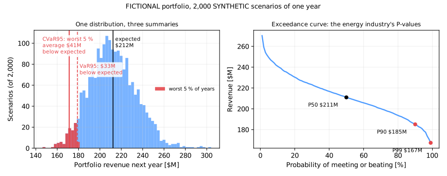
Histogram of 2,000 synthetic years with VaR and CVaR marked, and the exceedance curve with P50, P90 and P99

Summary	Value
Expected revenue	$212M
Standard deviation	$22M
P50 / P90 / P99	$211M / $185M / $167M
VaR95 (below expected)	$33M
CVaR95 (below expected)	$41M
CVaR99 (below expected)	$51M

The distribution is skewed. The good tail stretches further than the bad one, because price spikes and the batteries add upside. So the mean sits above the median, and a symmetric "±2 standard deviations" would misjudge both tails.

9 · Implementation¶

from energy_or.risk.measures import cvar, euler_contributions, exceedance, value_at_risk
from energy_or.risk.scenarios import driver_shapley, risk_scenarios

sc = risk_scenarios(2_000, seed=13)  # SYNTHETIC: 2,000 settled years
R = sc.portfolio / 1e6  # $M per scenario
loss = R.mean() - R
print(exceedance(R, 0.9), value_at_risk(loss, 0.95), cvar(loss, 0.95))

by_asset = sc.by_asset / 1e6
contrib = euler_contributions(by_asset.mean(axis=0) - by_asset, 0.95)
phi = driver_shapley(lambda s: cvar(s.portfolio.mean() - s.portfolio, 0.95) / 1e6)

10 · Solve: who and what causes the bad years¶

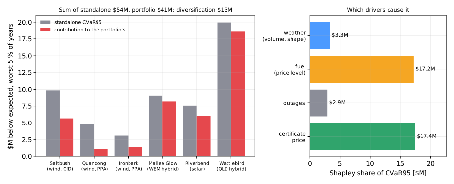
Standalone CVaR against contribution to the portfolio's CVaR by asset, and Shapley shares of CVaR by driver

By asset. Add up the six assets' CVaRs as if each were owned alone and you get $54M. The portfolio's is $41M: $13M of diversification. The contributions show where the portfolio's bad years come from:

Asset	Mean [$M]	Standalone CVaR95 [$M]	Contribution [$M]	Why
Saltbush Plains (wind, CfD)	38.0	9.9	5.7	25 % merchant; outages; the CfD covers 75 %
Quandong Ridge (wind, PPA)	22.2	4.8	1.1	95 % sold as produced: only volume risk is left
Ironbark Gully (wind, PPA)	12.9	3.1	1.4	80 % contracted
Mallee Glow (WEM hybrid)	34.7	9.0	8.2	All merchant; a different market, so little diversification
Riverbend Sun (solar)	30.1	7.5	6.1	Half merchant, solar-shaped prices
Wattlebird Bay (QLD hybrid)	74.5	19.9	18.6	Merchant solar and certificates; the battery earns most when prices are high

Quandong's standalone risk is $4.8M, almost all outage risk, but it adds only $1.1M to the portfolio. Its outages rarely coincide with the portfolio's bad years. The Queensland hybrid is the opposite: it is bad when the portfolio is bad. Risk is a property of the portfolio, not of an asset. An asset's standalone risk answers "should I buy it alone?". Its contribution answers "what does it do to what I already own?".

By driver. Switch drivers on and off with common random numbers and share out CVaR with the Shapley value (as Chapters 9 and 12 shared out losses and gains):

Driver	Share of CVaR95
Certificate price	$17.4M
Fuel / price level	$17.2M
Outages	$2.9M
Weather (volume and shape)	$3.3M

Two lessons:

Independent risks add like variances, not like dollars. Weather on its own moves revenue by several million dollars a year, but next to two larger and independent price risks it adds little to the tail. The biggest driver dominates. Halving a small risk changes little; halving a big one changes a lot.
Most of this portfolio's risk is price risk, and price risk can be hedged. About 1.4 million certificates a year are sold at spot, and about 1.4 TWh of merchant generation (plus the batteries' spread) floats with the price level. Both can be sold forward. Outages and wind volume cannot be hedged with a swap. That sets up Chapter 14.

11 · Interpret¶

Budget on the P50 of $211M, not the expected $212M. The difference is the upside skew.
Debt sized on a P90 year of $185M, or on a P99 of $167M for a lender who wants that. The difference between the two, $18M a year, is the price of the lender's extra confidence.
In a bad year (the worst 5 %), revenue is on average $41M below expected. In those years the average fuel multiplier is 0.76, the average certificate price is $16, and 43 % of them contain a major outage (25 % of all years do).
The riskiest asset by contribution is the Queensland hybrid. The safest is the PPA farm, whose buyer has taken the price risk. As Chapter 12 showed, the buyer pays for that with a strike below the farm's merchant value.

12 · Backtest: how much should we trust these numbers?¶

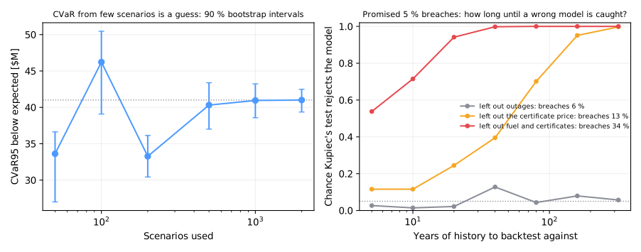
CVaR estimated from few scenarios with bootstrap intervals, and the power of Kupiec's test against wrong models

Sampling error. A CVaR95 from 100 scenarios rests on the worst 5 of them. The left panel draws random subsets and bootstraps each: - from 50 or 100 scenarios, the estimate ranges from $34M to $46M; - at 50 and at 200 scenarios, even the 90 % interval misses the 2,000-scenario value (the bootstrap cannot invent tail scenarios the sample does not contain); - the numbers settle only with 1,000 or more scenarios.

A risk number should always travel with its sample size, and never with more decimal places than that supports.

Is the model right? The standard check is a VaR backtest: count the years in which realised revenue fell below the model's P95 (a breach). A correct model breaches in 5 % of years. Kupiec's (1995) proportion-of-failures test asks whether the observed breach rate is consistent with 5 %:

\[ \mathrm{LR} = -2\ln\!\big[(1-p)^{n-x}p^{x}\big] + 2\ln\!\big[(1-\hat p)^{n-x}\hat p^{x}\big] \sim \chi^2_1, \qquad \hat p = x/n . \]

We play nature with a fresh set of 2,000 "realised" years and test three wrong models, each built by an analyst who left a driver out:

Model left out	P95 it promised	Real breach rate	Chance the test catches it with 10 years	with 40 years
nothing (correct model)	$179M	5.1 %	—	—
outages	$180M	5.5 %	1 %	13 %
certificate price	$188M	12.7 %	12 %	40 %
fuel and certificate price	$202M	33.8 %	71 %	100 %

An annual risk model cannot be validated from annual history. Ten years of data will not catch a model whose 1-in-20 year actually arrives every 8 years. This is why risk teams backtest on daily or monthly profit and loss, where there are hundreds of observations, and why they review a model's assumptions (is every driver in?) rather than wait for the data to prove it wrong. (The power curve has small kinks at low $n$ because breach counts are whole numbers.)

13 · Adding realism¶

Correlation between drivers. Here fuel, weather and certificates are independent. In reality a gas shock and a calm winter can arrive together, and certificate prices fall when a lot of new renewables connect. Copulas or a factor model (McNeil, Frey and Embrechts, 2015) add this; tail dependence makes CVaR larger.
Counterparty risk. A PPA removes price risk only while the buyer pays. Add a small annual default probability for each offtaker, with replacement at the merchant price.
Regulatory risk. The certificate scheme has an end date, loss factors are revised every year, and market price caps change. Treat each as a scenario driver with expert-elicited probabilities.
Multi-year horizons. Lenders care about consecutive bad years. Draw paths, not independent years, and look at the minimum DSCR along each path.
Model risk. Run the whole chapter with two different weather libraries and report the spread.

14 · Exercises¶

Guided

Compute CVaR90 and CVaR99 of the portfolio and of each asset. Does the ranking of assets by contribution change with $\alpha$? Why might it?

Engineering

risk_scenarios loops over scenarios in Python. Profile it and vectorise the settlement for the as-produced contracts. How many scenarios a second can you reach, and does the CVaR estimate change by more than its bootstrap interval?

Market

Raise the certificate price's standard deviation to $15 and lower its mean to $20, closer to a market near the end of a certificate scheme. Re-run the driver Shapley. Which assets' contributions move most?

Challenge

Show from the LP in section 7 that the Euler contribution $q \cdot L_i$ equals the derivative of portfolio CVaR with respect to scaling part $i$, when the tail is unique (no ties at VaR).

Production challenge

Design the monthly risk report: which numbers, with which intervals, and which backtest. Specify how many monthly observations Kupiec's test needs to detect a 12.7 % breach rate with 80 % power, using kupiec_power.

15 · Production perspective¶

The scenario engine is a product. Version it, seed it, and log every driver's parameters with each risk report. A change in CVaR must be traceable to a change in an input.
One settlement. The risk model, the budget and the finance system must settle contracts with the same code. Reconcile the P50 to the budget every month.
Report intervals and sample sizes, not lone numbers.
Backtest at the frequency you have data for (daily or monthly P&L), and review the driver list annually. The biggest model errors are missing drivers.
Limits. A risk limit (for example "CVaR95 below $45M") is a constraint. Check it with the same engine before any new contract is signed. Chapter 14 builds that check into an optimiser.

Run it yourself¶

Artefact	Location
Risk measures: VaR, CVaR (exact and LP), Euler, bootstrap, Kupiec	`src/energy_or/risk/measures.py`
Scenario engine and driver Shapley	`src/energy_or/risk/scenarios.py`
The fictional portfolio and its settlement	`src/energy_or/data/portfolio.py`
Tests	`tests/test_risk.py`
Notebook	`notebooks/13_how_bad_can_a_year_get.ipynb`