11 · Cycle, augment or rest? Planning a battery's life
Intermediate Advanced Case B MILP · DP · duality Decisions under uncertainty

In this chapter
- Put the whole life of a battery into one model: market revenue, cycling, fade, the warranty allowance, a capacity contract and augmentation
- Solve it four ways:
- a MILP (exact, with duals that explain every year)
- dynamic programming (a decision for every possible state)
- rules of thumb
- rolling re-planning
- Read the answer as a chain of marginal values: the revenue of the next cycle, the value of a MWh of capacity, and the wear cost that links them
- Turn the life plan into the wear cost for tomorrow's bids, and backtest that it beats both "cycle whenever it pays today" and "cycling is too expensive"
- Backtest the policies against uncertain markets and fade, knowing only the past, and measure what re-planning is worth
- Drag the levers yourself in an interactive explorer
A battery that trades "whenever there's a spread" is spending something it can't buy back cheaply. Each cycle uses capacity and warranty allowance and brings the next augmentation closer. A battery that hoards cycles leaves money on the table every day. Somewhere between is a rate of use where the next cycle earns exactly what it costs the future. This chapter finds it for every year of a battery's life, decides when to buy capacity back, and shows how that one number, the wear cost, should discipline the bids the battery submits every five minutes.
1 · The real-world problem
The owner of the Case B battery (10 MW / 20 MWh) has three linked commitments:
- A capacity contract. The battery earns $400k a year as long as its year-end capacity test shows at least 18 MWh of usable energy. This could be a network support or firming agreement.
- A warranty with a throughput allowance of 72 GWh over ten years (Chapter 10).
- A market that pays for cycles, with diminishing returns (Chapter 10's revenue curve), drifting down about 3 % a year as more batteries arrive.
Usable energy fades with time and use. Strings can be added in 2.5 MWh blocks at a cost that falls about 6 % a year, plus $300k per campaign for cranes, outage and commissioning.
The questions: how hard should it cycle each year? When should it augment, and by how much? And what wear cost should the bidding software use tomorrow?
2 · The physical system: how the pieces connect
          throughput B (MWh/yr) ──► market revenue m·R(B)   (concave: Chapter 10)
               │
               ├──► wear: −κ·B MWh of capacity              (κ ≈ 7×10⁻⁵ MWh/MWh)
               ├──► warranty allowance: Σ B ≤ 72 GWh in years 0–9
               ▼
  usable energy E ──► calendar fade −c·E per year           (c ≈ 0.96 %)
               │
               ├──► capacity contract: pays C if E ≥ 18 MWh at year end
               ├──► throughput cap: B ≤ 365 × 1.6 cycles × E
               ▲
  augmentation: + 2.5 MWh blocks at p_y $/MWh + F per campaign
Every arrow is a trade-off. Cycling earns money but uses capacity and allowance. Capacity keeps the contract and allows cycling, and can be bought back. Augmentation costs money but restores both.
3 · The decisions
Each year \(y\): the throughput \(B_y\) (equivalently, cycles per day) and the number of blocks \(n_y\) to add at the start of the year.
4 · Variables
| Symbol | Meaning | Type |
|---|---|---|
| \(E_y\) | usable energy at the start of year \(y\) [MWh] | continuous |
| \(B_y\) | energy discharged in year \(y\) [MWh] | continuous |
| \(n_y\) | augmentation blocks added | integer 0–4 |
| \(z_y\) | a campaign happens | binary |
| \(w_y\) | the contract test passes | binary |
5 · Objective
Here \(m_y\) is the market level, \(R\) the concave revenue curve, \(b = 2.5\) MWh, \(\delta = 1/1.08\), and \(s\) a salvage value per MWh left at the end.
6 · Constraints
7 · Formulation: why it's a MILP, and why that's fine
Why these techniques? Structure → method
| Property of the problem | Here | So |
|---|---|---|
| Revenue against throughput | concave, piecewise linear (the Chapter 10 curve) | epigraph variables \(t_y \le m_y(\alpha_k + \beta_k B_y)\): linear, with no binaries |
| Lumpy decisions | blocks of 2.5 MWh, a fixed cost per campaign, a contract paid only if energy ≥ 18 MWh | integer \(n_y\) and binaries \(z_y, w_y\): a MILP |
| Other constraints | fade, cycling cap and warranty allowance are linear | linear rows, so the integers are the only difficulty |
| Size | 15 years, 45 integer variables, about 300 constraints | branch and bound proves optimality in about a second |
| Time coupling | one state, usable energy \(E_y\), carries from year to year | dynamic programming on a grid of \(E\) |
| Prices of resources | a MILP has no duals | fix the integers, re-solve the LP, read the duals |
| Uncertainty | market ±15 % a year, fade ±20 % | not in the MILP: re-plan every year and test by Monte Carlo |
Chosen. - The MILP, because the decisions really are whole numbers and the fixed cost is what makes augmenting happen in bursts. It returns a plan with a proof of optimality. - The epigraph form of the revenue curve. Because revenue is concave and we maximise, the solver picks the binding segment itself. A non-convex curve would need binaries. - Dynamic programming, as a check and as a policy. It matched the MILP to 0.01 % ($19.866M against $19.868M) and gives the right decision at any energy level, which a single plan does not. - A paired Monte Carlo backtest, because a plan that is optimal for the forecast can still lose to a rule when the forecast is wrong.
Not chosen. - LP relaxation, then rounding. The campaign cost and the contract test are what the model is about. Rounding can miss the contract line or split a fixed cost. - A rule of thumb alone. It tied the optimiser in the base case, because its thresholds were read off the plan. When the contract changed, it lost $1.2M to $1.7M. - A scenario-tree stochastic programme. It is the principled answer to uncertainty, but trees grow exponentially. Annual re-solving captures most of the value, and perfect information is worth only $0.4M. - A metaheuristic. The exact model is small enough that it is never needed, and it could not provide a gap or duals.
What the theory guarantees. - Branch and bound returns a proven optimum of the piecewise-linear model, or a bound on how far it can be. - DP is optimal up to its grid. Both rely on the Bellman principle: the best plan from any year onwards does not depend on how the battery got there. - MILPs have no strong duality, so the duals are those of the LP with the integers fixed. They are valid for that augmentation schedule, not for changing it.
References. - Wolsey (2021), Integer Programming: formulation strength, fixed-charge and indicator constraints (Chapter 5). - Bertsekas (2017), Dynamic Programming and Optimal Control: the DP check, and Bellman (1957) in Choosing a technique and the simplex method. - Land and Doig (1960), An automatic method of solving discrete programming problems: branch and bound (same section).
See Further reading, Chapter 11 and Choosing a technique.
Everything is linear except the integers. The concave revenue curve becomes linear by the epigraph trick, \(t_y \le m_y(\alpha_k + \beta_k B_y)\) for every segment \(k\), and maximising \(t_y\) picks the right segment. The fixed campaign cost needs a binary \(z_y\); the contract needs a binary \(w_y\); blocks are integers. That's 45 integer variables and about 300 constraints. HiGHS solves it in about a second.
8 · Visualisation: one optimal life, four views
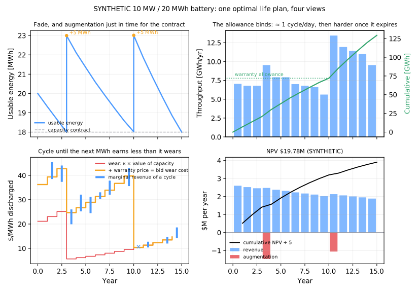
Read the four panels together:
- Energy (top left) fades about 0.7 MWh a year. The plan augments 5 MWh in year 3 and again in year 10, each time in the year the capacity test would otherwise fail. It never buys capacity earlier than needed, because new energy gets cheaper every year and capacity above the contract line is worth far less.
- Throughput (top right): about one cycle a day for ten years. Exactly 72 GWh are used by year 10, so the warranty allowance binds. Once the warranty expires, the battery cycles 1.4–1.6 times a day.
- Marginal values (bottom left): every year, the revenue of the next cycle (blue) equals the wear cost (orange). That is the optimality condition in picture form.
- Cash (bottom right): revenue declines with the market, and the two augmentation years dip. NPV is $19.78M.
9 · Implementation
from energy_or.bess.augmentation import LifeModel, plan_life

plan = plan_life(LifeModel())  # SYNTHETIC parameters
print(plan.explain())
plan.dispatch_wear_cost(0)  # the wear cost tomorrow's bids should use [$/MWh]
explain() prints the year-by-year rationale:
 yr  E start  aug  E after  throughput  EFC/d  contract  marg. rev  wear cost  why
  0    20.00    0    20.00       7,038   0.96       met     $ 36.2  $    36.2  cycle until marginal revenue = wear cost + warranty price
  2    18.65    0    18.65       6,792   1.00       met     $37–44  $    42.7  cycle until marginal revenue = wear cost + warranty price
  3    18.00    2    23.00       9,529   1.14       met     $20–26  $    24.7  augment 5 MWh; cycle until marginal revenue = wear cost + warranty price
 10    18.01    2    23.01      13,440   1.60       met     $ 10.7  $    10.4  augment 5 MWh; cycling limited by energy: capacity is the bottleneck
10 · Solve: the price of a cycle, derived
Re-solve the LP with the integers fixed and read the duals.
- Value of capacity. \(\mu_{y+1}\), the dual of the fade equation, is what one more MWh of usable energy at the end of year \(y\) is worth to the rest of the life.
- Warranty price. \(\omega\), the dual of the warranty allowance, is what one more MWh of allowance is worth.
Where \(0 < B_y <\) cap, the KKT conditions say:
The right-hand side is the wear cost: what the next MWh discharged really costs. It isn't a property of the cells alone. It depends on where the battery is in its life:
| Year | Value of 1 MWh of capacity | Wear \(\kappa\mu\) | + warranty | Bid wear cost |
|---|---|---|---|---|
| 0 | $302k | $21.1 | $15.1 | $36.2/MWh |
| 2 (contract test looming) | $359k | $25.1 | $17.6 | $42.7/MWh |
| 3 (just augmented) | $81k | $5.7 | $19.0 | $24.7/MWh |
| 10 (warranty over) | $148k | $10.4 | — | $10.4/MWh |
Why capacity is worth $360k one year and $81k the next
Just before an augmentation, the battery sits on the contract line. Every MWh it wears must be bought back next year (≈ $230k/MWh plus a share of the campaign) or the contract lapses. Right after augmenting, it has 5 MWh of headroom, and a MWh worn now only brings the next campaign a little closer. The same cycle costs twice as much in year 2 as in year 3, so the plan cycles less in year 2 and more in year 3. A fixed degradation cost can't do that.
The other techniques, for comparison
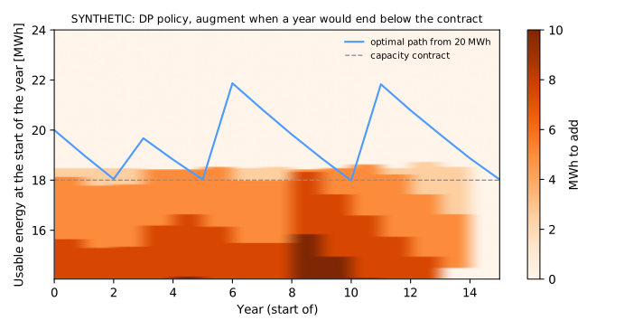
Dynamic programming solves the same problem backwards on a grid of usable energy:
Without the warranty allowance (which would add a second state, cumulative throughput), DP finds $19.866M against the MILP's $19.868M, with the same augmentation schedule. That is a 0.01 % discretisation error. Where the MILP gives one plan with duals, DP gives a policy: the right decision for any energy level in any year. The map shows the rule the optimum follows: augment when this year would otherwise end below the contract, and by the smallest amount that clears it for several years.
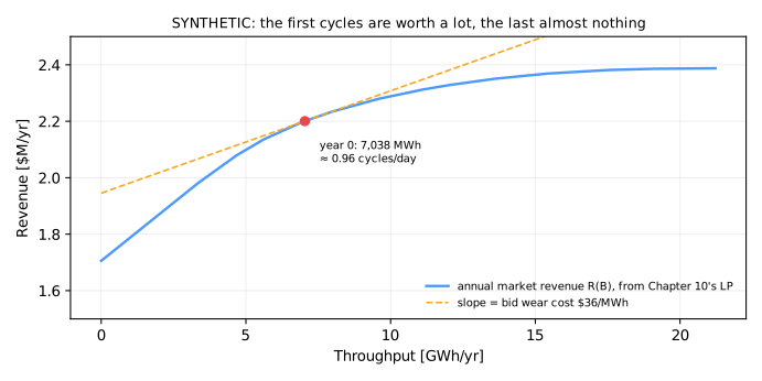
Chapter 10 found the price of a cycle as the slope of revenue against throughput within a month. Here the same curve, annualised, meets the cost side, and the optimum sits where its slope equals the wear cost.
What moves the plan
| Case | NPV | Augmentation (years) | Year-0 bid wear cost | Year-0 cycles/day |
|---|---|---|---|---|
| Base | $19.78M | 5 MWh (3), 5 MWh (10) | $36.2/MWh | 0.96 |
| No augmentation allowed | $18.61M | — (contract lost 11 of 15 years) | $58.3/MWh | 0.75 |
| No warranty allowance | $19.87M | 2.5 (2), 5 (5), 5 (10) | $17.8/MWh | 1.54 |
| No contract, no salvage | $17.39M | none | $23.5/MWh | 1.31 |
| Contract doubled to $800k | $23.47M | same as base | $36.2/MWh | 0.96 |
| New energy 50 % cheaper | $20.41M | same as base | $36.2/MWh | 0.96 |
Two lessons hide in this table:
- Augmentation makes cycling cheaper. Forbid it, and every MWh worn is lost for good. The wear cost jumps to $58, the battery cycles 22 % less, and it still loses the contract by year 4.
- The warranty allowance is the binding constraint in the base case. Remove it and the battery cycles 1.5 times a day from day one, and the wear cost halves. A doubled contract or cheaper cells change the NPV but not the decisions: the plan was already protecting the contract at the lowest-cost timing.
11 · Interpret: from a life plan to tomorrow's bids
The plan says year 0's wear cost is $36/MWh. Feed it to the bidding controller (Chapter 9's rolling MPC) as \(k_{deg}\), and compare with other choices. Each run is scored by its lifetime value: revenue over a synthetic week, minus the plan's wear cost for every MWh discharged.
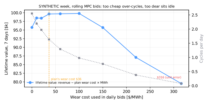
Seven synthetic days, rolling MPC bids (Chapter 9), only the wear cost changed:
| Wear cost in the bids | Revenue | Discharged | Cycles/day | Lifetime value |
|---|---|---|---|---|
| $0 (every spread) | $109,213 | 357 MWh | 2.55 | $95,751 |
| $20 | $109,111 | 276 MWh | 1.97 | $98,421 |
| $36 (the plan's) | $108,619 | 229 MWh | 1.63 | $99,640 |
| $60 | $106,961 | 181 MWh | 1.29 | $99,692 |
| $100 | $105,464 | 137 MWh | 0.98 | $99,785 |
| $150 | $100,215 | 108 MWh | 0.77 | $95,713 |
| $316 (the unit error) | $79,505 | 11 MWh | 0.08 | $79,526 |
The lifetime value has a broad plateau from about $36 to $100/MWh, where everything scores within 0.2 % because few trades have margins in that range. It falls away on both sides: - $0 cycles 2.5 times a day and gives up 4 % of lifetime value, despite earning the most revenue. - $316 sits almost idle and gives up 20 %.
The plan's number lands on the plateau without any tuning. This rich synthetic week pays well enough that, even at $36, the battery cycles faster than the plan's year-average of one a day. That is correct: cycle when it pays. Next year's re-plan sees the extra throughput.
Willy-nilly versus rationed
With no wear cost the battery takes every spread. It looks best on the week's revenue line and is worst for the asset, because it spends capacity and warranty allowance on trades worth less than they cost. With the guide's $316/MWh it barely moves and forfeits most of the energy market. The plan's wear cost is the price that rations cycles to the trades that pay for themselves over the life. Re-compute it as the plan updates, because it changes with the contract margin, the warranty and the market.
12 · Backtest: does planning beat a rule of thumb when the future surprises?
The plan above assumes it knows the market and the fade rate. It doesn't. The
backtest draws 60 futures: the market follows a random walk around its trend (15 %
a year), and the fade rate is uncertain by ±20 % (1σ). Each policy decides every year
from what it has seen so far: the energy measured at the last test, the allowance
used, and this year's market. It is the same discipline as Chapter 9's
historical_only.
- Never augment, cycle once a day.
- Rule of thumb: when energy falls below 18.5 MWh, top it back up to 20.
- Plan once at year 0 and follow it whatever happens (open loop).
- Re-plan every year with the MILP from the measured state (rolling horizon).
- Perfect information: the plan made knowing each future (the ceiling).
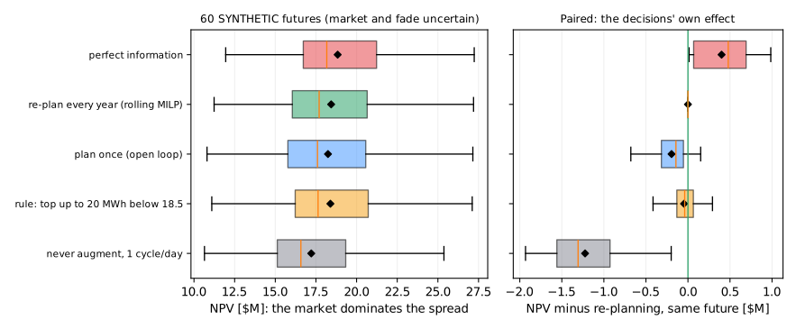
Sixty synthetic futures, paired: every policy faces the same futures, so differences are measured precisely.
| Policy | Mean NPV | p10 – p90 | vs re-planning (mean ± 2 s.e.) |
|---|---|---|---|
| Never augment, 1 cycle/day | $17.21M | $12.6M – $20.7M | −$1.22M ± 0.11 |
| Rule: top up to 20 MWh below 18.5 | $18.39M | $13.6M – $22.2M | −$0.05M ± 0.05 |
| Plan once, never revise | $18.24M | $13.5M – $22.2M | −$0.20M ± 0.05 |
| Re-plan every year | $18.44M | $13.6M – $22.3M | — |
| Perfect information (ceiling) | $18.84M | $13.9M – $22.5M | +$0.40M ± 0.08 |
What this says, and what it doesn't:
- Augmenting at all is worth $1.2M. It is the biggest decision in the table.
- A plan you never revise loses $0.2M to one you re-solve as the battery and the market reveal themselves. The fade rate is uncertain by ±20 %, and an open-loop plan augments in the wrong year when the battery ages faster or slower than assumed.
- Perfect foresight would add only $0.4M (2 %). That caps what any better market or degradation forecast could be worth to this decision.
- The rule of thumb ties with the optimiser here, and that's no accident. Its thresholds (top up below 18.5, about a cycle a day) were read off the optimiser's plan. That is how good operating rules are made. But a rule is only as good as the conditions it was tuned for. Change them, and the same 24 futures tell a different story:
| Policy, vs re-planning | Contract removed | Contract needs 19 MWh |
|---|---|---|
| Rule (unchanged) | −$1.74M ± 0.14 | −$1.22M ± 0.13 |
| Plan once | −$0.01M ± 0.01 | −$0.30M ± 0.14 |
Without the contract, the rule keeps buying capacity nobody pays for. With a stricter contract, it tops up too little and loses the contract. The optimiser adapts because it re-derives the decision from the economics. That is the case for optimising rather than following a rule: the optimiser finds the rule, explains it, and re-tunes it when the world changes.
13 · Adding realism
- Fade is not linear. Calendar fade depends on SOC and temperature, and cycle fade on depth (Chapter 10's rainflow model). The linear κ is a local approximation. Re-plan when the Kalman filter moves.
- Augmentation and the warranty. Adding strings may change the supplier's warranty terms, or need their consent. Model it as a constraint or a cost, and never assume it away.
- Mixed cohorts. New strings are healthier than old ones. Usable energy is then limited by the weakest string (Chapter 10), and balancing or separate cohorts may matter.
- Stochastic programming. The rolling MILP is certainty-equivalent. A scenario-tree MILP or stochastic DP (with the market as a state) would value the option to wait explicitly (Toolbox T8).
- Replacement versus augmentation. At some point the inverters, not the cells, are the bottleneck. Add a repowering decision.
14 · Exercises
Guided
For a one-year life with a linear revenue slope \(r\), show that the battery cycles
flat out if \(r > \kappa s/(1+i)\) and not at all otherwise. Check it against
plan_life (the tests do).
Engineering
Make the yearly re-plan a scheduled job: read the latest Kalman SOH and throughput counters, solve, write the year's wear cost where the bidding service reads it, and alert if it moves by more than 20 %.
Market
Raise the contract to $800k/yr. When does the plan augment, and what happens to the wear cost in the year before each campaign? Try it in the explorer.
Challenge
Add cumulative throughput as a second DP state and solve with the warranty allowance. Compare the policy maps with and without it.
Production challenge
The market drops 30 % in one year. Run the rolling policy through that scenario,
and explain each of its decisions from explain() as you would to an investment
committee.
15 · Production perspective
- The life plan is a slow loop around the fast loop. It is re-solved yearly or quarterly; the bidding MPC runs every 5 minutes. They communicate through one number, the wear cost, with its provenance logged.
- Explain every recommendation. For an augmentation, give the contract year it protects, the cost, and the alternative. For a cycling rate, show marginal revenue against wear.
- Backtest the planner, not just the bidder: against uncertain futures, with only the information each year would have had.
Try it: the battery life explorer
Pick a rule and see the whole life respond. The dashed green line is the optimiser's plan for comparison. The readout compares your year-0 cycling with the optimiser's wear cost, so you can see whether you are over- or under-cycling.
Run it yourself
| Artefact | Location |
|---|---|
Life model, MILP plan with duals and explain(), DP, policies, Monte Carlo |
src/energy_or/bess/augmentation.py |
| Interactive explorer (same model, kept in sync by a test) | docs/assets/javascripts/battery-life-explorer.js |
| Tests | tests/test_bess_augmentation.py |
| Notebook | notebooks/11_planning_a_battery_life.ipynb |