T2 · Does an optimum exist, and is it unique?¶

Intermediate Optimisation toolbox Case A

In this chapter

The three things that can happen to an LP: optimal, infeasible, unbounded, and the theorems that say why
Turn "infeasible" into a diagnosis: how far from feasible, and which constraints conflict (an irreducible infeasible subsystem)
See when the optimum is not unique, map the whole set of optimal solutions, and choose one by a stated rule
Find degenerate points where the shadow price is a range, not a number, and watch solvers disagree there
Recognise ill-posed problems, where a cent changes the answer by 50 MW, and fix them with regularisation

Chapter 1 always got a clean answer: one dispatch, one shadow price. Real models don't always behave. A contract minimum that can't be met makes the problem infeasible. A missing constraint makes it unbounded. Two farms worth the same make the answer arbitrary. A value that crosses another flips 50 MW in one interval. Each is a question about the mathematics of the problem, not about the solver, and a senior optimiser recognises all of them.

1 · The real-world problem¶

The same two farms and 100 MW connection, one interval at a time. A site manager asks four questions, and each needs a theory answer:

Question	Theory
"The model says infeasible. What do I tell the trader?"	existence; infeasibility certificates
"Why did the solver give WF_B 80 MW and not 50?"	uniqueness; optimal faces
"What is the connection worth per MWh right now?"	duality; degeneracy
"Why did the plan swing 50 MW when the price moved a cent?"	well-posedness; regularisation

2 · The physical system¶

Behind the shared limit $L$, farm $i$ can export up to $A_i$ MW, is worth $v_i$ per MWh, and may have a firm minimum $m_i$ (a contract or an operating rule):

\[ \max_P \ \sum_i v_i P_i \quad \text{s.t.}\quad \sum_i a_i P_i \le L,\qquad m_i \le P_i \le A_i . \]

3 · The decision¶

The dispatch $P$, as in Chapter 1. The new decision is about the model: is its answer meaningful, and if not, what do we change?

4 · Existence: three outcomes and two theorems¶

Every LP ends in exactly one of three states: optimal, infeasible (no point satisfies the constraints) or unbounded (the objective can grow forever).

Fundamental theorem of LP. If an LP is feasible and bounded, an optimum exists, and one is attained at a vertex of the feasible region. That is why simplex methods only visit vertices.
Weierstrass. A continuous function on a closed, bounded, non-empty set attains its maximum. Physical bounds ($0 \le P_i \le A_i$) make the feasible set bounded, so a physically complete model always has an optimum if it has any feasible point.

So "unbounded" almost always means a constraint is missing, and "infeasible" means the requirements contradict each other or the data.

Infeasible: measure it, then explain it¶

Give WF_A a firm minimum of 40 MW and WF_B 75 MW, behind a 100 MW limit. HiGHS says infeasible, which is true and useless. Two better answers:

How far from feasible? The elastic (phase-one) problem adds a shortfall $s_i \ge 0$ to each minimum and minimises $\sum_i s_i$. The answer is 15 MW: 40 + 75 − 100.
Which constraints conflict? A deletion filter removes constraints one at a time and keeps a removal whenever the rest are still infeasible. What remains is an irreducible infeasible subsystem (IIS): here {limit, WF_A minimum, WF_B minimum}. Remove any one and the problem is feasible.

Commercial solvers compute an IIS for you; the deletion filter shows what they do.

Unbounded: a missing constraint¶

Give WF_B a coefficient of −0.5 in the limit (a unit that relieves the constraint, like a load or a unit on the other side of the line) and forget its availability bound. Each extra MW of WF_B makes room for half a MW more of WF_A, both earn money, and nothing stops it: HiGHS says unbounded. Physically impossible; mathematically correct. Unbounded is a modelling bug report.

5 · Uniqueness: when many dispatches are equally good¶

Make both farms worth $65/MWh. Every dispatch on the edge from (20, 80) to (70, 30) earns the same $6,500/h:

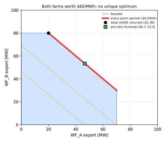
Equal values: a whole edge of optimal solutions

The solver returns one vertex, (20, 80), but nothing in the model prefers it. Ask a different solver, or reorder the variables, and you may get (70, 30). Telling WF_A it was curtailed "because the optimiser said so" is not defensible here.

Mapping the optimal set. Solve once for the optimal value $z^*$. Then, for each farm, minimise and maximise its output subject to the constraints and $\sum_i v_i P_i \ge z^* - \varepsilon$:

Farm	Output over all optimal solutions
WF_A	20 to 70 MW
WF_B	30 to 80 MW

A zero-width range for every variable means the optimum is unique. Chapter 1's case, $50 and $80/MWh, gives exactly (20, 80).

Choosing one, on purpose. Lexicographic optimisation keeps the first objective at its optimum and then optimises a second one. Here the second objective is "closest to pro-rata by available MW", an LP that minimises the largest deviation. It returns (46.7, 53.3): same value, and a rule you can explain.

When is an LP optimum unique?

At an optimal vertex, if every non-basic variable has a strictly non-zero reduced cost, the optimum is unique. A zero reduced cost means the objective is parallel to an edge, as with equal values here. Strictly convex objectives (Section 7) are always unique.

6 · Degeneracy: when the shadow price is a range¶

Set WF_A to 40 MW and WF_B to 60 MW available, with values $50 and $80/MWh, and a 100 MW limit. Both farms run flat out and the limit is exactly full: three constraints meet where two would do. That vertex is degenerate.

Optimal value against the limit

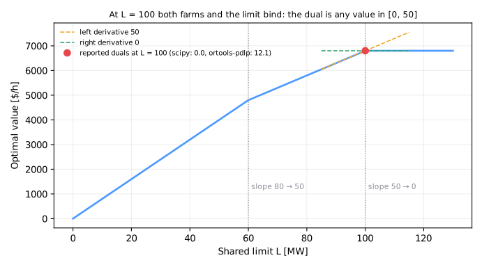
The optimal value is a piecewise-linear function of the limit, and its slope is the shadow price:

Below 100 MW, one MW less costs WF_A's $50: the left derivative is 50.
Above 100 MW, one MW more is worth nothing, because both farms are already full: the right derivative is 0.
At exactly 100 MW, any value in [0, 50] is a valid dual. The simplex solvers (HiGHS, GLOP, CLP) stop at a vertex and report 0; PDLP, a first-order method that need not stop at a vertex, reports 12.1. None of them is wrong.

Move the limit to 99.999 MW and every solver reports 50 again. Before quoting a shadow price, check it is not degenerate: compare the left and right derivatives (limit_derivatives) or ask two solvers.

7 · Ill-posedness: a cent that moves 50 MW¶

Hadamard called a problem well-posed if a solution exists, is unique, and depends continuously on the data. Case A fails the third test at a tie:

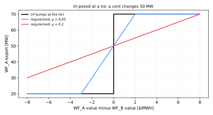
The LP's answer jumps at a tie; regularisation makes it a ramp

When WF_A's value crosses WF_B's, the LP moves 50 MW in one step. The forecast error on a spot price is many dollars, so a decision that flips on a cent is a decision driven by noise.

Regularisation. Add a small quadratic penalty:

\[ \max_P \ \sum_i v_i P_i - \frac{\mu}{2} \sum_i P_i^2 \quad\text{s.t. the same constraints.} \]

The objective is now strictly concave, so the optimum exists, is unique, and is Lipschitz in the values: a farm's dispatch moves by at most $1/\mu$ MW per $/MWh change in a value (half that here, where two farms share the limit). The KKT conditions give the solution in closed form, $P_i = \mathrm{clip}\big((v_i - \nu a_i)/\mu,\ 0,\ A_i\big)$, with the limit's price $\nu \ge 0$ found by bisection ("water-filling"). There is no solver call at all.

It costs a little value:

Value gap (WF_A − WF_B)	LP	μ = 0.05	μ = 0.2
$0	any split earns $6,500/h	50 / 50, $0 lost	50 / 50, $0 lost
$1	70 / 30	60 / 40, $10/h lost	52.5 / 47.5, $17.50/h lost
$5	70 / 30	70 / 30, $0 lost	62.5 / 37.5, $37.50/h lost

Small μ gives a stable decision near ties and the LP's answer away from them.

8 · Visualisation¶

The three figures above are the chapter's pictures: the optimal edge (non-uniqueness), the kink (degeneracy) and the step versus the ramp (ill-posedness).

Why these techniques?¶

Why these techniques? Structure → method¶

Property of the problem	Here	So
Question	not "what is the optimum?" but "does one exist, is it unique, can we trust its duals?"	diagnostic tools around a solver, not a new solver
Model	two continuous MW, one shared-limit row, two availability bounds	tiny enough to draw, and to solve many times
Infeasible	firm minimums that sum past the limit	an elastic (phase-one) LP for how far; a deletion filter for which constraints
Unbounded	a missing bound on a relieving unit	read it as a modelling bug; check the bounds
Non-unique	equal values give a whole optimal edge	optimal ranges by min and max LPs, then a lexicographic tie-break
Degenerate	three constraints meet at a vertex where two would do	left and right derivatives of the value in the limit, and two solvers
Ill-posed	a cent can move 50 MW	add a strictly concave term: regularisation, solved in closed form by KKT and bisection
Speed	every tool is a handful of tiny LPs	cost is irrelevant; clarity decides

Chosen. - The elastic LP adds a shortfall $s_i \ge 0$ to each minimum and minimises their sum. It is the same device as the artificial variables of phase one of the simplex method: their total measures how infeasible the model is (T0). - The deletion filter finds an irreducible infeasible subsystem with one solve per constraint. Commercial solvers do this internally; the filter shows how. - Min and max LPs over the optimal face (objective held within $\varepsilon$ of the optimum) give honest ranges for every variable. - A quadratic penalty makes the optimum unique and Lipschitz in the data.

Not chosen. - Trusting the solver's single answer. It is one vertex of an optimal edge, and it changes with variable order or solver. - Random perturbation of the objective to break ties. It gives one answer, but not one that anyone can explain to a curtailed farm. - The interior-point centre of the optimal face. It is unique and defensible, but it is not a rule an operator can state, unlike "closest to pro-rata". - A nonlinear solver for the regularised problem. The KKT conditions give the solution as a clipped formula, so bisection on one price replaces the solver.

What the theory guarantees. - A feasible, bounded LP has an optimum at a vertex (fundamental theorem), and a continuous objective on a closed, bounded set attains its maximum (Weierstrass). A strictly concave objective on a convex set has at most one optimum, and with $\mu > 0$ the dispatch moves by at most $1/\mu$ MW per $/MWh. At a degenerate vertex the dual is an interval, and every value in it is valid.

References. - Chinneck (2008), Feasibility and Infeasibility in Optimization: finding out why a model is infeasible and what to relax (T2). - Chinneck and Dravnieks (1991), Locating minimal infeasible constraint sets: the irreducible infeasible subsystem (T2). - Bertsimas and Tsitsiklis (1997), chapters 2-4: vertices, degeneracy and the optimal face (Chapter 1). - Charnes (1952), Optimality and degeneracy in linear programming: degeneracy and artificial-variable penalties (Choosing a technique). - Choosing a technique for how structure picks the method.

9 · Implementation¶

from energy_or.toolbox.wellposed import (
    IntervalLP,
    solve_interval,
    elastic_feasibility,
    irreducible_conflict,
    optimal_ranges,
    tie_break_pro_rata,
    limit_derivatives,
    regularised_dispatch,
)

firm = IntervalLP(values=(50, 80), available_mw=(70, 80), limit_mw=100, min_mw=(40, 75))
solve_interval(firm).status  # 'infeasible'
elastic_feasibility(firm)  # (15.0, [0, 15])
irreducible_conflict(firm)  # ['limit', 'min_0', 'min_1']

tie = IntervalLP((65, 65), (70, 80), 100)
optimal_ranges(tie)  # [[20, 70], [30, 80]]
tie_break_pro_rata(tie)  # [46.7, 53.3]

limit_derivatives(IntervalLP((50, 80), (40, 60), 100))  # (50.0, 0.0): degenerate
regularised_dispatch((66, 65), (70, 80), 100, mu=0.05)  # [60, 40]

10 · Solve¶

Situation	Status	What the theory says
Chapter 1 ($50 and $80, 70 and 80 MW)	optimal, unique	(20, 80), dual $50
Firm minimums 40 + 75 MW	infeasible	15 MW short; IIS = limit + both minimums
Relieving unit, no bound	unbounded	a missing constraint
Equal values	optimal, not unique	WF_A anywhere in 20–70 MW
Both farms full, limit full	optimal, degenerate	dual anywhere in [0, 50]
Values within a cent	optimal, ill-posed	50 MW swing; regularise

11 · Interpret¶

The lesson

"Optimal" is not the end of the analysis. Ask four more questions of every model: does an optimum exist (and if not, which constraints conflict), is it unique (and if not, which rule picks one), is the dual unique (or is the point degenerate), and does the answer depend continuously on the data (or does noise decide it). A model that can answer all four can be explained to a control room.

12 · Backtest¶

Ill-posedness shows up in a backtest as churn: dispatch that flips between farms from one interval to the next with no economic reason. Counting large swings per day is a cheap first metric for the backtesting framework (Milestone 7). Whether regularisation reduces them depends on how often values sit near a tie: on Chapter 1's synthetic day only 5 of 288 intervals come within $1 of it, and the regularised plan, which moves smoothly with every price change, makes more moderate swings than the LP. Measure churn on real data before choosing μ.

13 · Adding realism¶

Numerical conditioning. Mixing MW and W, or coefficients of 10⁻⁶ and 10⁶ in one row, makes LPs numerically ill-posed: solvers warn, or stop on tolerances. Scale the model (units in names, Code rules).
IIS in commercial solvers. Gurobi and CPLEX compute an IIS directly; HiGHS reports infeasibility. The elastic model works everywhere and gives a size, not just a set.
Uniqueness in MIPs. T1's whole-turbine schedules show the same issue with integers: many schedules earn the same.
Regularisation elsewhere. The same idea appears as ridge regression (T3) and as penalties on ramping in dispatch.

14 · Exercises¶

Guided

For $A = (40, 60)$ and $L = 100$, compute the optimal value at $L = 99$ and $L = 101$ by hand, and so the left and right derivatives.

Engineering

Write a check that runs after every solve and warns when the optimum is not unique (non-trivial optimal_ranges) or the limit's dual is degenerate.

Market

WF_A is merchant at spot × 0.92 + $15; WF_B is a $65 PPA. At what spot price is the model ill-posed? How often does Chapter 1's synthetic day come within $1 of it?

Challenge

Prove that the regularised dispatch is Lipschitz in the values with constant $1/\mu$ (per farm), using the KKT conditions.

Production challenge

The trader sees "infeasible" at 05:00. Design the message the system sends instead: the shortfall size, the conflicting constraints, and the least-bad relaxation.

15 · Production perspective¶

Never ship "infeasible" alone. Ship the elastic shortfall and the conflicting constraints.
Treat "unbounded" as a failed deployment. It means a constraint is missing.
Log uniqueness and degeneracy flags with every decision, so a shadow price is never published at a degenerate point.
Regularise decisions that drive physical actions, so the plant doesn't hunt between two equally good set-points every five minutes.

Run it yourself¶

Artefact	Location
Existence, uniqueness, degeneracy, regularisation	`src/energy_or/toolbox/wellposed.py`
Tests	`tests/test_toolbox.py`
Notebook	`notebooks/t2_existence_uniqueness.ipynb`