14 · Hedging the portfolio: what to sell forward, and how much¶

Intermediate Advanced Case L Least squares · QP · CVaR LP · duality · MILP · out-of-sample

In this chapter

Choose a hedge book for the fictional Lantern Bay portfolio from a menu of products: regional swaps, caps, certificate forwards, and more of each asset's output on PPAs
Solve one problem five ways and compare them:
- a rule of thumb
- least squares (the minimum-variance hedge)
- a bounded QP (Markowitz)
- the mean–CVaR LP (Rockafellar–Uryasev)
- a MILP that trades in whole lots
Read the LP's duals as stress probabilities: the bad years a hedge is priced against
Meet the optimiser's curse: a hedge tuned on too few scenarios over-promises, and only an out-of-sample test shows by how much

Chapter 13 measured the risk: the portfolio's CVaR95 is $41M, and about 85 % of it is price-level and certificate-price risk, which markets let you sell. This chapter decides how much to sell. The decision is small (14 numbers), but it shows clearly why the choice of objective matters more than the choice of solver.

1 · The real-world problem¶

Lantern Bay's trading desk can sell forward. The CFO wants a hedge book that: - protects the bad years (the board's limit is on revenue in a 1-in-20 year); - does not give away too much expected revenue to the counterparties; - avoids over-hedging: selling energy forward that the portfolio may not produce.

The obvious rule, "sell our expected output forward", is what many first hedge books do. Is it any good?

2 · The physical and market system¶

Hedges are financial. They settle against the regional price and never touch dispatch. All products and prices below are illustrative:

Product	Payoff per unit to Lantern Bay	Limit	Priced at
Swap (NSW, QLD, VIC)	sell 1 MW flat for the year: receive the fixed price, pay the regional price, every hour	0–250 MW	expected average price − $1.50/MWh
Buy cap ($300 strike)	receive $(p-300)^+$ every hour, pay a premium	0–150 MW	115 % of expected payout
Sell cap	the reverse	0–150 MW	90 % of expected payout
LGC forward	sell certificates at a fixed price instead of spot	up to the 1.38 million sold at spot	expected spot − $1
PPA (per asset)	sell more of the asset's output as produced, with certificates, at a fixed price	up to its uncontracted share	expected value − $3/MWh

Each counterparty charges a risk premium: it takes your risk, so it asks for part of your expected revenue. Every hedge therefore costs mean revenue, and the question is how much tail protection each dollar of cost buys.

Basis risk. Swaps settle on the regional price, but each asset is paid its own output at the regional price × loss factor. The WEM hybrid has no swap market here at all, and can only be hedged by selling its own output on a PPA.

3 · The decision¶

A vector $h$ of 14 volumes, one per product: MW for swaps and caps, thousands of certificates for the forward, share of output for each PPA.

4 · Variables¶

For scenario $s$ of the 2,000 from Chapter 13, the unhedged revenue is $R^0_s$ and product $j$ pays $P_{sj}$ per unit. Revenue is linear in the hedge:

\[ R_s(h) = R^0_s + \sum_j P_{sj}\,h_j . \]

That one line is why hedging is an optimisation problem with a friendly shape. Linear in $h$ means: - the mean is linear; - the variance is quadratic; - CVaR is LP-representable.

hedge_problem(sc) builds $R^0$ and $P$ from the scenario set.

5 · Objective: five answers to "what is a good hedge?"¶

Method	Objective	Problem class	Ignores
Rule of thumb	sell expected merchant volume per region, and all spot certificates	none	cost, correlation, volume risk
Minimum variance	$\min_h \operatorname{Var}[R(h)]$	least squares (T3)	cost, limits, which side of the mean
Mean–variance (Markowitz)	$\max_h \mathbb{E}[R] - \tfrac{\gamma}{2}\operatorname{Var}[R]$, within limits	bounded convex QP	asymmetry: good years count as risk
Mean–CVaR	$\max_h (1-w)\,\mathbb{E}[R] + w\,T_{95}(h)$, within limits	LP	— (only the bad tail is penalised)
Mean–CVaR in lots	the same, with $h_j$ in whole lots of 5 MW, 25,000 certificates or 5 %	MILP	—

Here $T_{95}$ is the tail revenue: the average revenue of the worst 5 % of years, which equals the expected revenue minus CVaR95 of the shortfall. With $w = 0.5$, a dollar of tail revenue is worth as much as a dollar of expected revenue.

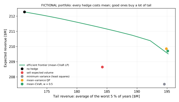
The board's version of the same problem is "maximise expected revenue, subject to tail revenue ≥ F". Sweeping F traces the efficient frontier.

6 · Constraints¶

Volume limits for every product (table above). You cannot sell more of an asset's output than is uncontracted, nor more certificates than you create.
No-arbitrage pricing. Buying and selling the same cap costs the bid–ask spread, so the optimiser never does both.
Lots (the MILP). Real trades come in standard sizes.

7 · Formulation: the mean–CVaR LP¶

Why these techniques? Structure → method¶

Property of the problem	Here	So
Revenue in terms of the hedge	$R_s(h) = R^0_s + \sum_j P_{sj} h_j$: linear in $h$	mean linear, variance quadratic, CVaR LP-representable
What the board fears	the worst 5 % of years, not variation in general	mean–CVaR, an LP (Rockafellar and Uryasev)
Size	2,000 scenarios, 14 products: 2,000 shortfall rows and 2,015 columns	HiGHS in about 0.2 s
Limits	volume bounds per product, no more than the uncontracted output	box constraints, which unconstrained least squares ignores
Trading costs	premia and bid–ask spreads	linear costs inside $P_{sj}$ and the objective
Trade sizes	5 MW, 25,000 certificates, 5 % of output	integers: a MILP, about 0.6 s
Estimation error	the optimum is fitted to the scenarios	judge out of sample; stability of the hedge as a diagnostic

Chosen. - Mean–CVaR as an LP. Revenue is linear in $h$, so the epigraph form of CVaR keeps the whole problem linear, with a global optimum and duals. - Least squares and the QP, but only as comparisons. Minimum variance is the right diagnostic of which products move with revenue. The bounded QP respects limits and lands close to the CVaR hedge here. - A MILP for lots, because real trades are whole lots. - A rule of thumb as the benchmark. DeMiguel et al. (2009) show simple splits can be hard to beat once estimation error counts.

Not chosen. - Minimum variance as the decision. It has the lowest standard deviation ($5.3M) and cannot be traded: it buys negative caps and sells 199 % of the WEM asset's output. - Mean–variance as the main tool. It works here because the hedged distribution is nearly symmetric. Where it is not, variance penalises good years. - Rounding the LP solution to lots. It can be infeasible or far from optimal when lots are large next to the volumes. The MILP avoids the risk. - Robust optimisation. It suits an uncertainty that can be bounded but not described. Here the scenarios describe it, and a worst case would sell everything.

What the theory guarantees. - The mean–CVaR problem is an LP, so HiGHS returns a global optimum. The frontier is concave, because the optimal value of an LP is concave in its right-hand side. The duals are the stress probabilities in section 11. - The MILP is proved optimal by branch and bound. - None of this holds out of sample. The in-sample optimum is biased upwards (Smith and Winkler, 2006): with 50 scenarios, $7M of promised tail revenue is not delivered.

References. - Rockafellar and Uryasev (2000) and Krokhmal, Palmquist and Uryasev (2002): CVaR in the objective and in constraints. - Markowitz (1952), Portfolio selection: the mean–variance trade-off. - DeMiguel, Garlappi and Uppal (2009), and Smith and Winkler (2006): naive splits and the optimiser's curse. - Bessembinder and Lemmon (2002): why forward prices carry a premium. - Conejo, Carrión and Morales (2010): CVaR for electricity producers.

Full entries are in Further reading, Chapter 14. See also Choosing a technique.

With variables $h$, a threshold $t$ and shortfalls $u_s$:

\[ \begin{aligned} \max_{h,\,t,\,u}\quad & (1-w)\,\frac{1}{S}\sum_s R_s(h) \;+\; w\Big(t - \frac{1}{(1-\alpha)S}\sum_s u_s\Big) \\ \text{s.t.}\quad & u_s \ge t - R_s(h), \quad u_s \ge 0, \qquad s = 1,\dots,S \\ & \ell_j \le h_j \le m_j . \end{aligned} \]

This is Chapter 13's CVaR LP, mirrored for revenue and with the hedge added as variables: 2,000 shortfall rows and 2,015 columns. HiGHS solves it in about 0.2 s. The lot version substitutes $h_j = \text{lot}_j \cdot n_j$ with integer $n_j$; it solves in about 0.6 s.

8 · Visualisation: the frontier¶

Efficient frontier of expected against tail revenue, with the rule of thumb, minimum variance, mean–variance and mean–CVaR hedges marked

Revenue distributions unhedged, with the rule of thumb and with the mean–CVaR hedge; and the volumes each method sells

9 · Implementation¶

from energy_or.risk.hedging import (
    hedge_problem,
    mean_cvar_hedge,
    mean_variance_hedge,
    min_variance_hedge,
    naive_hedge,
    no_hedge,
)
from energy_or.risk.scenarios import risk_scenarios

sc = risk_scenarios(2_000, seed=13)  # SYNTHETIC
pb = hedge_problem(sc)  # R0 and the payoff matrix P, in $M
best = mean_cvar_hedge(pb, alpha=0.95, tail_weight=0.5)
board = mean_cvar_hedge(pb, tail_floor=190.0)  # max mean s.t. tail ≥ $190M
lots = mean_cvar_hedge(pb, tail_weight=0.5, lots=True)  # MILP
for name, volume, unit in best.table(pb):
    print(f"{name:28s} {volume:10.2f} {unit}")

10 · Solve: five hedges compared¶

Method	Expected [$M]	Std dev [$M]	Tail revenue [$M]	P90 [$M]	What it sells
No hedge	212.3	21.8	171.3	185.1	—
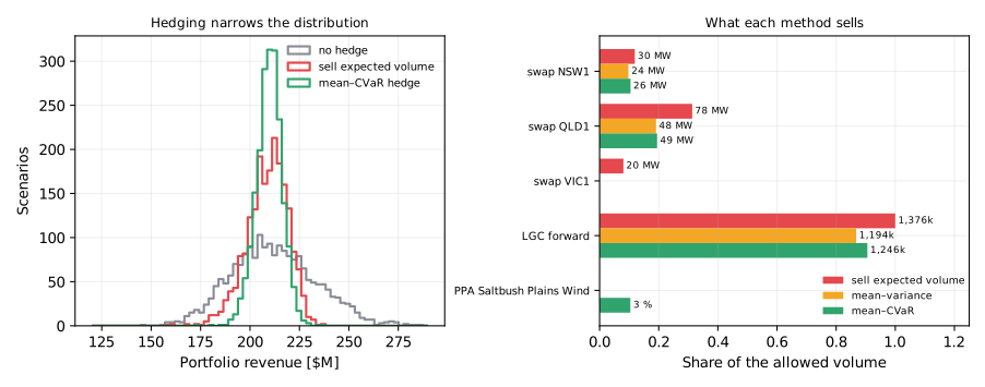
Sell expected volume	208.7	10.3	184.2	195.4	30 / 78 / 20 MW of NSW / QLD / VIC swaps; all 1.38 M certificates
Minimum variance (least squares)	207.5	5.3	194.5	200.4	infeasible: negative cap purchases, 199 % of the WEM asset's output
Mean–variance QP (γ = 0.05)	209.9	6.9	194.9	201.1	24 / 48 MW NSW / QLD swaps; 1.19 M certificates
Mean–CVaR LP (w = 0.5)	209.7	6.6	195.1	201.3	26 / 49 MW NSW / QLD swaps; 1.25 M certificates; 3 % of Saltbush on a PPA
Mean–CVaR MILP (lots)	209.8	6.7	195.1	201.2	25 / 50 MW; 1.25 M certificates

The rule of thumb gives up $3.6M of expected revenue and gains $13M of tail revenue. The mean–CVaR hedge gives up $2.6M and gains $24M. The rule's mistakes:

Over-selling Queensland. It sells 78 MW of flat swap against a solar-heavy asset whose battery already profits from high prices (a natural hedge). The swap's floating leg is paid in every high-price hour, including evenings the solar never sees.
Selling Victoria at all. The two Victorian wind farms are already 75 % and 95 % contracted.
Selling every certificate. The last few certificates cost more in premium than they save in the tail.

Least squares finds the lowest variance (sd $5.3M), but the answer cannot be traded. It buys a negative amount of caps, sells 199 % of the WEM hybrid's output and ignores the premium on every product. It is the right diagnostic (it shows which products move with revenue) and the wrong decision. T3's lesson, that the model is only as good as its loss function, applies again here.

Mean–variance and mean–CVaR land close together on this problem, because after hedging the distribution is nearly symmetric. They differ where the tail is asymmetric: variance penalises the good years too, and CVaR does not.

Lots cost almost nothing here. The MILP rounds the NSW swap down and the QLD swap up, and drops the 3 % PPA, which is smaller than a 5 % lot. Rounding is not always this harmless. When lots are large relative to the volumes, or a limit binds, rounding an LP solution can be infeasible or far from optimal, and solving the MILP is the safe way.

The frontier (first figure) is concave, which is typical. The first $9M of tail protection costs $0.7M of expected revenue. The last $3M of tail costs about $0.9M.

11 · Interpret: the duals are stress probabilities¶

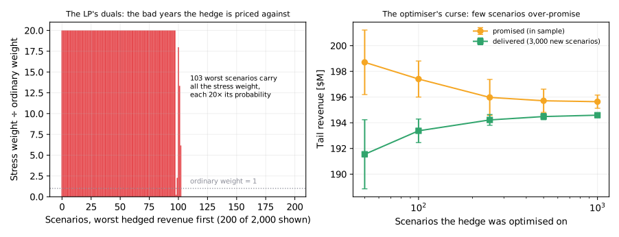
Stress weights from the LP duals across scenarios, and promised against delivered tail revenue as the number of scenarios grows

The duals of the 2,000 shortfall rows, normalised, form a probability vector $q$. It puts weight 20 (= 1/0.05) times the ordinary probability on each of the 103 worst hedged scenarios, and zero everywhere else. Under $q$ the world is the bad tail. LP duality then gives a clean rule for every product $j$ traded strictly inside its limits:

\[ (1-w)\,\underbrace{\mathbb{E}_p[P_j]}_{\text{expected cost}} \;+\; w\,\underbrace{\mathbb{E}_q[P_j]}_{\text{value in bad years}} \;=\; 0 . \]

A hedge is bought until what it costs on average equals what it pays in the bad years. For the Queensland swap at the optimum: - it costs $18.7k per MW-year on average (the premium); - it pays $18.7k per MW-year in the stress scenarios; - with $w = 0.5$, the two balance exactly.

The tests check this condition for every interior product. Products at zero, such as the caps and most PPAs, cost more on average than they return in the bad years, which is why they were not used.

The stress scenarios also show what is left after hedging. Before the hedge, the worst 5 % were years of low fuel prices (average multiplier 0.76) and cheap certificates ($16). After it, they average fuel 0.92 and certificates $28, close to normal, but 75 % of them contain a major outage. The hedge has sold the price risk, and what remains is operational risk, which swaps cannot touch. The tools for that are insurance (business-interruption cover), spares and maintenance strategy (Chapters 3–5).

12 · Backtest: the optimiser's curse¶

An optimiser picks the hedge that does best on the scenarios it was given. With few scenarios it finds hedges that fit those scenarios' quirks, and its reported tail revenue is optimistic. Smith and Winkler (2006) called this the optimiser's curse. The right panel of the figure solves the hedge on random subsets of a 3,000-scenario pool, then evaluates each hedge on 3,000 new scenarios:

Scenarios used	Tail revenue promised (in sample)	Tail revenue delivered (out of sample)	Spread of the QLD swap volume
50	$198.7M	$191.5M ± 2.7	± 24.5 MW
100	$197.4M	$193.4M ± 0.9	± 13.7 MW
250	$196.0M	$194.2M ± 0.4	± 11.0 MW
1,000	$195.6M	$194.6M ± 0.1	± 5.4 MW
all 3,000	—	$194.7M	—

With 50 scenarios the optimiser promises $7M more tail revenue than it delivers, and the recommended QLD volume swings by ±25 MW from one sample to the next. Two practical rules follow:

Always judge a hedge out of sample, on scenarios it was not fitted to.
Stability is a diagnostic. If re-running with a new seed moves the recommendation by more than a trade lot, there are not enough scenarios, or the objective is too flat to be worth acting on.

13 · Adding realism¶

Multi-period hedging. Real books hedge 1–3 years ahead in quarterly products, layering trades over time. That makes it a multi-stage stochastic programme (Birge and Louveaux, 2011): today's trade, then re-hedge as information arrives.
Shaped products. Solar-shaped and evening-peak swaps fit a solar-and-battery asset better than flat ones. Add them as columns of $P$.
Credit and collateral. Exchange-traded swaps need margin, and a bad price year ties up cash, which the Chapter 7 lenders care about. Add a constraint on the worst-case margin call.
Volume risk products. Weather derivatives and proxy-revenue swaps pay when the wind does not blow. They target what remains after this chapter's hedge.
Robust hedging. Replace the scenario average with a worst case over an ambiguity set of distributions (distributionally robust optimisation). It is another answer to the optimiser's curse.

14 · Exercises¶

Guided

Re-solve with tail_floor from $175M to $195M and plot the swap volumes against the floor. Which product enters first, and why does that make sense from its dual condition?

Engineering

mean_cvar_hedge builds a dense 2,000 × 2,015 matrix. Rewrite it with scipy.sparse and time both at 10,000 scenarios.

Market

Add a solar-shaped NSW swap (10:00–16:00) as a product. How much of the flat swap does it replace, and what happens to the tail revenue?

Challenge

Prove that at the optimum of the LP every product strictly inside its limits satisfies $(1-w)\mathbb{E}_p[P_j] + w\,\mathbb{E}_q[P_j] = 0$. Start from the Lagrangian and the reduced cost of $h_j$.

Production challenge

Specify the pre-trade check: before the desk executes any trade, re-run the portfolio CVaR with the new position, compare it with the limit, and log the result. What latency budget does it need if traders want an answer in under five seconds?

15 · Production perspective¶

Mark-to-market daily. Re-price the book against forward curves, and recompute CVaR with the hedge in place. A hedge chosen in January is not optimal in June.
OptOps for the hedge optimiser. For every run, log the solver status, solve time, the binding limits, the dual check from section 11, and the in-sample vs out-of-sample tail. Alert when they diverge.
The recommendation is an input to a human decision. Report the frontier, the stability across seeds, and what each trade does to the bad years. Do not report one optimal number.
Governance. Hedging limits, approved products and counterparties belong in a policy the board signs. The optimiser works inside that envelope, never around it.

Run it yourself¶

Artefact	Location
Products, market view, rule, least squares, QP, CVaR LP/MILP, frontier, out of sample	`src/energy_or/risk/hedging.py`
Scenario engine (Chapter 13)	`src/energy_or/risk/scenarios.py`
Tests	`tests/test_risk.py`
Notebook	`notebooks/14_hedging_the_portfolio.ipynb`

Property of the problem	Here	So
Revenue in terms of the hedge	\(R_s(h) = R^0_s + \sum_j P_{sj} h_j\): linear in \(h\)	mean linear, variance quadratic, CVaR LP-representable
What the board fears	the worst 5 % of years, not variation in general	mean–CVaR, an LP (Rockafellar and Uryasev)
Size	2,000 scenarios, 14 products: 2,000 shortfall rows and 2,015 columns	HiGHS in about 0.2 s
Limits	volume bounds per product, no more than the uncontracted output	box constraints, which unconstrained least squares ignores
Trading costs	premia and bid–ask spreads	linear costs inside \(P_{sj}\) and the objective
Trade sizes	5 MW, 25,000 certificates, 5 % of output	integers: a MILP, about 0.6 s
Estimation error	the optimum is fitted to the scenarios	judge out of sample; stability of the hedge as a diagnostic