16 · Robust against the constraint you did not forecast

Intermediate Advanced Case J · Case B Robust LP · Bertsimas–Sim budgets · cutting planes · DR-CVaR

In this chapter

• Five batteries hold back headroom so that, after a line trips, they can push flow off the lines that would otherwise overload. The corridor can then export more before the fault: a virtual transmission line.
• The scheme only works if the batteries respond. Decide, for a season:
  • how many MW to hold back on each battery;
  • how much more the zone may export;
  • how far to trust the batteries.
• Solve it four ways and compare them:
  • a robust LP with a Bertsimas–Sim budget of uncertainty ("at most \(\Gamma\) batteries fail"), by duality and by cutting planes;
  • a stochastic programme that prices an unrelieved overload (risk-based security, the Chapter 15 method);
  • distributionally robust CVaR: failure rates bounded by the data, dependence between failures unknown.
• Judge every design on a truth the planner did not model: a common-mode failure that takes out two batteries at once.

Chapter 15 planned for a distribution it trusted. This chapter is about the distributions you should not trust: a handful of trip records, 120 test activations, and an assumption that batteries fail independently. Robust optimisation asks a different question from stochastic programming: not "what is the expected cost?" but "what is the worst that can happen within limits I am willing to state?"

---

1 · The real-world problem

A renewable zone exports through a meshed corridor to three load centres. The network must be N−1 secure: after any single line trips, every remaining line must stay within its short-term rating. That rule caps the zone's export at 918 MW on a normal day, while the lines could carry 1,276 MW before a fault. Wind and solar beyond 918 MW are curtailed.

Five batteries sit downstream. If a line trips, they can discharge for a few minutes while generation in the zone is run back. That moves flow off the overloaded lines, so the network can allow more export before the fault. Large batteries run public schemes of this kind. Everything here, including the network, is fictional.

The scheme operator must decide for the coming season:

• how many MW to reserve on each battery, paid for with the trading value the battery loses (Chapter 15's recourse curve);
• how high to set the export limit, which changes daily with the line ratings;
• which batteries to arm for which trip.

The catch: a battery called on to respond might not. It might be offline, have lost communications, or have a protection setting that trips it. If it fails when a line has tripped, the overload is not relieved. Protection then trips the overloaded line, and the outage can cascade.

2 · The physical and market system

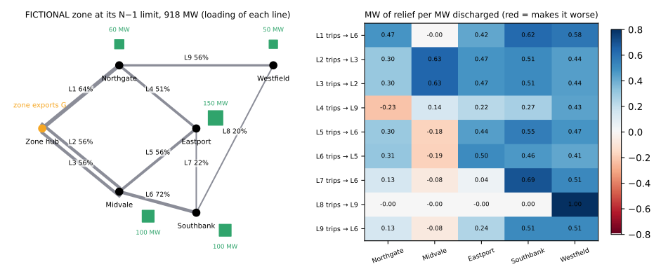
• Network (energy_or.data.virtual_line, fictional): six buses and nine lines, modelled with DC power flow (energy_or.network.dc_flow). A line trip changes the power-transfer distribution factors (PTDFs). The new factors are the coefficients of an outage constraint equation.
  • At 918 MW, Midvale–Southbank (L6) runs at 72 % of its rating.
  • If the hub–Northgate line (L1) trips, L6 picks up the flow and reaches its short-term rating (115 % of continuous). That is the limit that binds.
• Relief (right panel): MW taken off the worst post-fault line per MW a battery discharges, with the zone run back by the same amount.
  • Southbank and Westfield relieve almost every trip well.
  • Midvale relieves the L2/L3 trips best of all (0.63), but does nothing for the L1 trip (0.00) and makes four other trips worse (red). Injecting at Midvale pushes flow the wrong way.
• Batteries: 60, 100, 150, 100 and 50 MW, all 2-hour. Reserving costs trading value: \(\$397\) a day for the first MW of every 10 MW, rising to \(\$7{,}158\) a day for all of it (Chapter 15's curve, scaled by size and a local price factor).
• Day types: ratings are 5 % lower on 20 % of days and 10 % lower on 10 % of days (hot, still weather). The day's rating is known when the day's limit is set.
• Value of export: \(\$1{,}000\) per MW of extra limit per day (curtailment avoided, illustrative).
• What the planner knows:
  • Trips: 6 years of trip records. Some lines tripped twice in six years, so their rates are guesses.
  • Battery failures: 4 failures in 120 test activations, so \(\hat p = 3.3\,\%\) per call.
• What is true (used only to judge decisions):
  • Batteries fail independently at 3 %.
  • Eastport and Southbank share a control gateway. With probability 2 % per call, they fail together.

3 · The decision

Stage	When	Decision	Knows
Season	before the season	\(x_i\): MW reserved on battery \(i\)	trip history, test results
Day	each morning	\(G_d\): export limit; \(u_{dki} \le x_i\): MW battery \(i\) is armed to give if line \(k\) trips	the day's line ratings
Event	seconds after a trip	nothing: the scheme fires	which line tripped, not which batteries will respond

4 · Variables

• \(x_i \in [0, P_i]\): MW reserved on each of 5 batteries for the season.
• \(G_d \ge 0\): export limit on day type \(d\) (3 types).
• \(u_{dki} \in [0, x_i]\): arming, for each day type, trip \(k\) (9 lines) and battery: 135 variables.

5 · Objective

Maximise the expected value of the export minus the trading value the batteries lose:

\[ \max\; \sum_d \pi_d\, v\, G_d \;-\; \sum_i C_i(x_i), \]

where \(\pi_d\) is the share of days of type \(d\), \(v = \$1{,}000\) per MW-day, and \(C_i\) is battery \(i\)'s convex, piecewise-linear reservation cost. The results report the gain over no scheme, \(\$899{,}815\) a day of export at the unaided limits.

6 · Constraints

• Pre-fault: every line within its continuous rating, derated on the day.
• Post-fault: for every trip \(k\), every surviving line \(e\) and both directions,

[ h_{ke}\, G_d \;+\; \sum_i a_{kei}\, \delta_i\, u_{dki} \;\le\; (1 - \rho_d)\, r_e , ]

where \(h_{ke}\) is the post-fault flow per MW exported, \(a_{kei}\) the flow per MW battery \(i\) discharges (negative means relief), \(r_e\) the short-term rating and \(\rho_d\) the day's derate. - \(\delta_i \in \{0, 1\}\) is whether battery \(i\) responds. It is not known when \(G_d\) and \(u\) are set. How to handle \(\delta\) is the whole chapter.

There are 144 post-fault rows per day type. Only one binds at the optimum: after L1 trips, L6. That gives a closed form you can check by hand,

\[ G = \frac{r_{L6} + \text{guaranteed relief}}{h_{L1,L6}} = \frac{483 + \text{relief}}{0.526}. \]

With no batteries, \(483 / 0.526 = 918\) MW.

7 · Formulation

Why these techniques? Structure → method

Property of the problem	Here	So
Uncertainty	which batteries respond: \(2^5\) patterns, rare failures	a set of patterns, or a distribution over them
What is known about it	120 tests, 6 years of trips, no data on joint failures	a set you can defend more easily than a distribution
Where it enters	coefficients of the post-fault rows (\(a_{kei}\,\delta_i\)), row by row	constraint-wise robust LP (Soyster, 1973; Ben-Tal and Nemirovski, 1999)
How much to protect	"any one battery may fail" is a standard engineers already use (N−1)	a budget of uncertainty \(\Gamma\) that stays an LP (Bertsimas and Sim, 2004)
Consequence of failure	an unrelieved overload: a cascade, not a price	a guarantee (robust), or a penalty if you can price it (stochastic)
Probabilities	failure rate estimated, dependence unknown	distributionally robust risk over every distribution consistent with the data (Delage and Ye, 2010; Wiesemann, Kuhn and Sim, 2014)
Size	5 + 3 + 135 decisions, 432 post-fault rows	every method solves in well under a second

Chosen. - The Bertsimas–Sim robust counterpart. Each row must hold whatever any \(\Gamma\) of its relieving batteries do. The worst case of a sum of at most \(\Gamma\) terms is an LP in its own right. Its dual turns the robust row into a few linear rows, so the whole problem stays an LP. - Cutting planes, the same problem solved without the dual. Solve, ask an adversary for each row's worst \(\Gamma\) failures, add those rows, and repeat (Mutapcic and Boyd, 2009). It must reach the same optimum, which is a check on the reformulation. - Risk-based security: the Chapter 15 machinery, with a penalty per MW of unrelieved overload, weighted by the estimated probability of every (day, trip, pattern) scenario. - Distributionally robust CVaR: CVaR of the unrelieved overload, at its worst over every joint distribution of failures in which no battery fails more often than \(\bar p\). The data bound the rates; nothing bounds the dependence.

Not chosen. - Soyster's box, all five batteries failing at once (\(\Gamma = 5\)). It is computed, but only to show that the box prices the scheme at zero. - Ellipsoidal uncertainty (Ben-Tal and Nemirovski). It gives a second-order cone programme and suits many small, roughly normal errors. Five on/off failures are neither. - Chance constraints (P(overload) ≤ \(\epsilon\)). With discrete failure patterns they need binaries, or a convex approximation. CVaR is that approximation, and it is used here. - A total-variation ambiguity set around the estimated distribution. It moves \(\epsilon\) of probability onto "all five batteries fail", which kills the scheme at \(\epsilon = 1\,\%\). A set built from what the data say (failure rates) is easier to defend. - Adjustable robust optimisation, where the arming reacts to which batteries are online. Real schemes do this to some degree. It is section 13's first item.

What the theory guarantees. - For any \(\Gamma\), the robust design is feasible for every response pattern in which at most \(\lfloor\Gamma\rfloor\) of a row's relieving batteries fail. That is exact and needs no distribution. If failures are independent with probability \(p\), a row can fail only if more than \(\lfloor\Gamma\rfloor\) of its \(n\) batteries fail, which has probability \(P(\text{Bin}(n, p) > \Gamma)\). - Bertsimas and Sim also give a bound that holds for any independent, symmetric deviations. Here it is loose: 0.5 at \(\Gamma = 1\) with \(n = 4\). Battery failures are rare and one-sided, not symmetric. - The reformulation and the cutting-plane method reach the same optimum. The adversary's problem is an LP with integral corners, so a finite number of cuts suffices. - If the true distribution lies in the DR ambiguity set, the DR objective is a lower bound on the design's true value. That rests on Sion's minimax theorem, which lets the worst case and CVaR's inner minimum swap.

References. Further reading, Chapter 16 and Choosing a technique.

The robust row, by duality

For one row with relieving batteries \(J\) and possible relief losses \(\hat a_i u_i = |a_i|\,u_i\), the worst case of at most \(\Gamma\) failures is

\[ \beta(u, \Gamma) = \max_{w}\Big\{\sum_{i\in J}\hat a_i u_i\, w_i \;:\; \sum_i w_i \le \Gamma,\; 0 \le w_i \le 1\Big\}. \]

This is an LP in \(w\). Its dual is \(\min\{\Gamma z + \sum_i p_i : z + p_i \ge \hat a_i u_i,\; z, p \ge 0\}\). Strong duality lets the minimum replace the maximum inside a "≤" row, so the robust row becomes

\[ h G + \sum_i a_i u_i + \Gamma z + \sum_{i\in J} p_i \le (1-\rho) r, \qquad z + p_i \ge \hat a_i u_i,\; z, p \ge 0 . \]

That adds one \(z\) and one \(p_i\) per relieving battery to each row. The LP grows from 644 rows to 1,724, and stays an LP. With \(\Gamma = 0\) it is the nominal row. With \(\Gamma = |J|\) every relieving battery is assumed to fail: Soyster's box.

Cutting planes

Start from the nominal rows. At the current solution, the adversary takes each row's \(\lfloor\Gamma\rfloor\) largest losses \(\hat a_i u_i\) (and a fraction of the next). If the row breaks, add the row as it would be with those batteries failed. Repeat until nothing breaks.

The distributionally robust risk term

Let \(o\) be the unrelieved overload. With \(\text{CVaR}_\alpha(o) = \min_t\, t + \mathbb{E}[(o-t)^+]/(1-\alpha)\), the ambiguity set \(\mathcal{Q} = \{q : q(\text{battery } i \text{ fails}) \le \bar p_i\}\) and LP duality on the inner supremum, the worst case is

\[ \min_{t,\,\mu,\,\lambda \ge 0}\; t + \frac{\mu + \sum_i \lambda_i \bar p_i}{1-\alpha} \quad\text{s.t.}\quad \mu + \sum_{i \text{ fails in } f} \lambda_i \;\ge\; \sum_{d,k} \pi_{dk}\, (o_{dkf} - t)^+ \quad \forall f . \]

There is one row per response pattern. \(\lambda_i\) is the price of battery \(i\)'s failure rate: how much the worst case would grow if it failed a little more often.

8 · Visualisation

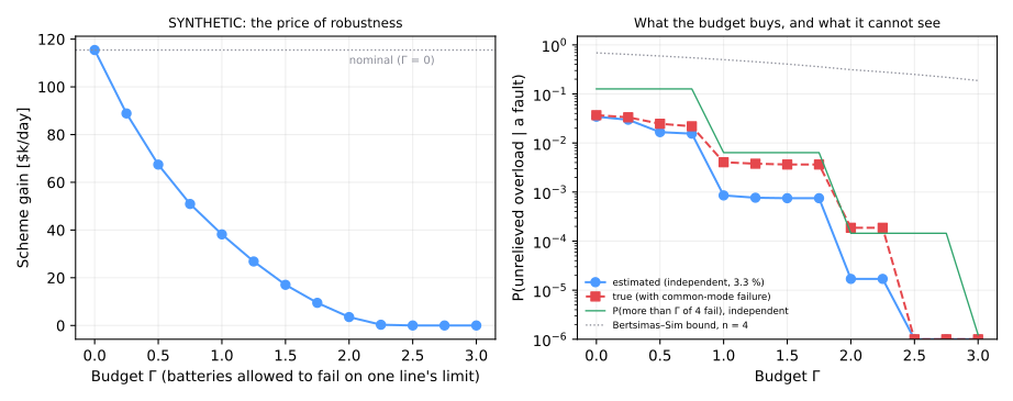
Left: the price of robustness. - Trusting every battery is worth $115k a day. - Guarding against any one failure (\(\Gamma = 1\)) keeps $38k. - Against two (\(\Gamma = 2\)) keeps $3.5k. - From \(\Gamma = 2.5\) the scheme is worth nothing.

Right: what each \(\Gamma\) buys. - The estimate (blue) drops by a factor of 40 at \(\Gamma = 1\). That is the step from "one failure breaks it" to "two failures break it". - The truth (red) drops only by a factor of 9. The common-mode failure is a double failure, outside the set \(\Gamma = 1\) protects. Robust optimisation kept its promise: any one failure is covered. What was wrong was the planner's belief that double failures are as rare as independence implies. - The Bertsimas–Sim symmetric bound (dotted) is true but useless here.

9 · Implementation

from energy_or.data import virtual_line as vl
from energy_or.data.battery_days import battery_days
from energy_or.risk.robust import (
    Zone,
    evaluate,
    failure_upper_bound,
    fault_events,
    reservation_cost_curve,
    solve_scheme,
)

cost = reservation_cost_curve(battery_days(1_000, seed=31))  # Chapter 15's recourse
zone = Zone(cost, value_per_mw_day=1_000.0)  # FICTIONAL network, SYNTHETIC data

# What the planner believes, and what is true.
est = fault_events(vl.fault_history() / 6, vl.TEST_FAILURES / vl.TEST_ACTIVATIONS)
truth = fault_events(
    vl.TRUE_FAULTS_PER_YEAR,
    vl.TRUE_FAILURE_PROBABILITY,
    common_mode=(vl.COMMON_MODE_PROBABILITY, vl.COMMON_MODE_PAIR),
)

nominal = solve_scheme(zone, "nominal")
robust = solve_scheme(zone, "budget", gamma=1.0)  # Bertsimas–Sim by duality
same = solve_scheme(zone, "cutting_plane", gamma=1.0)  # and by cutting planes
priced = solve_scheme(zone, "risk", events=est, overload_cost_per_mw=1e6)
cautious = solve_scheme(zone, "dr_cvar", events=est, failure_bound=4 / 120)
evaluate(zone, robust, truth).overload_events_per_season()

10 · Solve

Design	Export limit, normal day [MW]	Reserved [MW] (N, M, E, S, W)	Gain [$/day]	Overloads per season, estimated	… true
No scheme	918	0	0	0	0
Nominal (trust every battery)	1,206	54, 0, 105, 90, 45	115,437	0.097	0.101
Robust, \(\Gamma = 1\)	1,064	54, 0, 61, 41, 44	38,173	0.0024	0.011
Robust, \(\Gamma = 2\)	961	24, 0, 27, 18, 20	3,528	0.0000	0.0005
Risk-based, $1M per MW	1,177	48, 0, 75, 90, 45	111,779	0.085	0.092
Risk-based, $10M per MW	1,050	49, 0, 55, 37, 40	37,752	0.0022	0.010
DR mean, \(\bar p = \hat p = 3.3\,\%\)	1,149	42, 0, 75, 80, 35	105,881	0.084	0.092
DR mean, \(\bar p = 7.5\,\%\) (95 % bound)	1,034	24, 0, 15, 51, 20	63,784	0.045	0.060
DR-CVaR 90 %, \(\bar p = 3.3\,\%\)	930	0, 0, 0, 10, 0	7,714	0.011	0.020

An "overload per season" is a fault that leaves a line above its rating. The estimate uses the planner's trip rates and independent 3.3 % failures; the truth uses the true trip rates and the common-mode failure.

Check the robust design by hand. On the binding row (L1 trips, L6), the reserved batteries give 0.47 × 54, 0.42 × 61.2, 0.62 × 40.8 and 0.58 × 44.2 MW of relief: 25.4, 25.7, 25.3 and 25.6 MW. - The optimiser has made every battery equally important. Losing any one costs at most 25.7 MW, the least it can arrange. - Guaranteed relief is 102.0 − 25.7 = 76.3 MW, so \(G = (483 + 76.3)/0.526 = 1{,}063\) MW. - \(\Gamma = 2\) does the same at about 11.3 MW each.

Robustness here is diversification by design: no battery may carry more of the guarantee than the scheme can afford to lose.

Solve times. All are on a laptop, and every method is an LP. - Nominal: 644 rows, 0.01 s. - Robust reformulation: 1,724 rows, 0.02 s. - Cutting planes: 5 rounds, 674 rows, 0.03 s, with the same objective. - Risk-based: 13,454 rows over 864 scenarios, 0.08 s. - DR-CVaR: 14,350 rows, 0.25 s.

11 · Interpret

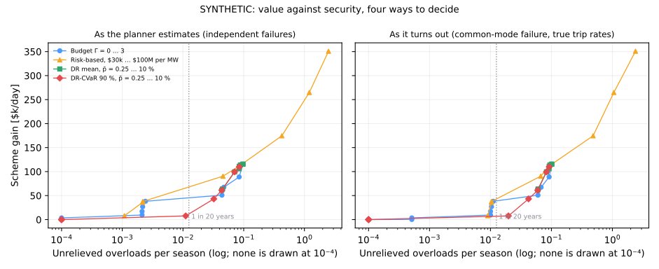
• Midvale is never used, whatever the method. Its relief on the one binding row is zero, and on four other trips it makes things worse.
• A budget is an implied price. \(\Gamma = 1\) and the risk-based design at $10M per MW of unrelieved overload are almost the same design. They differ by $421 a day and give the same true risk, about one overload in 90 seasons. Choosing \(\Gamma = 1\) says an unrelieved overload costs about $10M per MW.
• At $1M per MW, risk-based security runs the corridor much harder: 0.09 overloads a season, about one every 2.7 years. Whether that is acceptable is not an optimisation question. A reliability standard is a rule, not a price.
• A standard of one overload in 20 years is 0.0125 a season.
  • On the planner's estimate, \(\Gamma = 1\) meets it five times over (0.0024).
  • On the truth it only just meets it (0.011): the common-mode failure ate most of the margin.
  • \(\Gamma = 2\) meets it comfortably, at $35k a day less.
• The frontier:
  • In both panels, a well-priced risk-based design is about as efficient as any.
  • Distributionally robust designs sit slightly inside the frontier. They pay for worst-case dependence that, mostly, is not there.
  • That is not their purpose. Their purpose is section 12.

12 · Backtest: promised against delivered

Each method's own objective is a promise about what the design is worth. Judge every design on the truth, with an unrelieved overload costing $1M per MW:

Design	Promised [$/day]	Delivered on the truth [$/day]	Surprise
Nominal (promise valued at the estimate)	85,381	71,939	−13,441
Risk-based, $1M per MW	88,373	76,103	−12,271
Robust, \(\Gamma = 1\)	37,554	35,136	−2,418
DR mean, \(\bar p = 3.3\,\%\)	70,811	74,733	+3,922
DR mean, \(\bar p = 7.5\,\%\)	39,462	52,163	+12,701

1. The stochastic programme disappoints: it promised $88k and delivered $76k.
2. This is Chapter 14's optimiser's curse, with a cause you can name. The planner's model said Eastport and Southbank fail together with probability \(0.033^2 \approx 0.1\,\%\). The truth is 2 %.
3. The optimiser leaned on exactly those two batteries (75 and 90 MW reserved), because they relieve the binding row best.
4. The distributionally robust design keeps its promise. It delivered $75k against a promise of $71k.
5. It gave up $1.4k a day against the stochastic design on the truth, and in return its number could be signed.
6. With \(\bar p = 7.5\,\%\), the 95 % Clopper–Pearson bound from 4 failures in 120 tests, the truth lies inside the ambiguity set: each battery's true failure rate is at most 4.9 %. The DR objective is then a guaranteed lower bound on the true value (up to the trip mix, which is estimated). Here it is conservative by $12.7k.
7. The robust design kept its guarantee: every single failure is covered.
8. Its probability of failure was underestimated, as everyone's was.
9. Its loss on the truth is small because it had little left to lose.

Many small units. The price of robustness is steep here because each row has only four relieving batteries. Losing one loses a quarter of the relief. Build the same MW as many separately controlled units and a budget gets cheap. This is Bertsimas and Sim's central point: the protection needed grows like \(\sqrt n\), not \(n\).

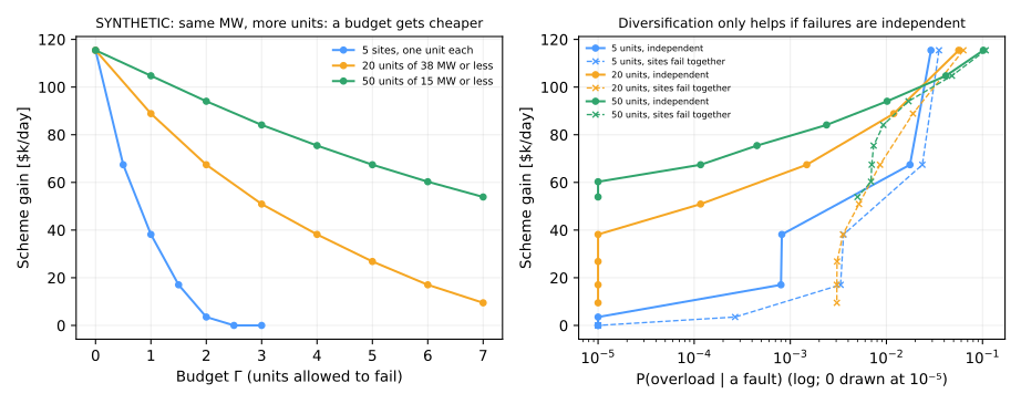
• 50 units of 15 MW or less: \(\Gamma = 4\) keeps $75k a day, with a 0.04 % chance per fault of an unrelieved overload when units fail independently.
• Five big batteries: \(\Gamma = 1\) keeps half as much, $38k, at twice the risk (0.08 %).
• But:
  • if a site's units all fail together (the dashed lines), diversification inside a site buys nothing;
  • the probability floors at 0.5–0.7 % for 50 units, whatever \(\Gamma\).
• Independence is the assumption every budget quietly rests on. Spread the scheme across sites, gateways and control systems before spreading it across more units.

13 · Adding realism

• Adjustable arming. Batteries report their status. Arm the ones that are online, so a battery known to be out is replaced before the fault, not after. Decision rules that react to observed status are adjustable robust optimisation (Ben-Tal et al., 2004).
• Planned outages. With a line out for maintenance, the next trip is an N−2 event with different PTDFs. Each outage gets its own day type and limits, and a season plan must cover the outage schedule, which itself changes.
• Partial response. A battery low on charge delivers part of its arming. Replace \(\delta_i \in \{0, 1\}\) by \(\delta_i \in [0, 1]\). The budget then counts lost fractions.
• Dynamic line ratings measured in real time instead of three day types.
• AC effects and stability limits. Voltage and transient stability bind before thermal limits on long corridors. The DC model cannot see them.
• The market. The export limit enters dispatch through constraint equations, priced by the market (Chapter 1's shadow prices). A higher limit lowers the zone's local price spread as well as its curtailment.

14 · Exercises

Guided

Solve the robust design for \(\Gamma = 0, 0.25, \dots, 2\) and, on the binding row, print each battery's relief \(|a_i|\,u_i\). Show that from \(\Gamma = 1\) the used batteries' relief is equal, and explain why with the dual variables \(z\) and \(p_i\).

Engineering

Time the reformulation and the cutting-plane method as the fleet is split into 5, 20, 50 and 100 units. Which grows faster, and why? Add a warm start to the cutting plane and measure again.

Market

At what value of export \(v\) does the \(\Gamma = 1\) scheme stop paying for itself? And at \(\Gamma = 2\)? Plot the break-even \(v\) against \(\Gamma\).

Challenge

Prove that the DR risk term with \(\alpha = 0\) and \(\bar p_i = \bar p\) for all \(i\) puts its worst-case probability on "every relieving battery fails together", and find the worst-case distribution when the \(\bar p_i\) differ.

Production challenge

Specify the scheme's monitoring: what is logged at every activation and test, how \(\hat p\) and its confidence bound are updated, how common-mode failures are detected (failures that coincide more often than independence allows), and what triggers a review of \(\Gamma\).

15 · Production perspective

• State the set, not just the answer. "Secure against any one battery failing" is a sentence an operator and a regulator can check. "Secure with probability 99.6 %" depends on a model of dependence nobody has validated.
• Measure dependence, not just failure rates. Count joint failures in tests and real events. A shared gateway, firmware version or protection setting is a common mode. The budget's guarantee is only as good as the claim that units fail separately.
• Report the promise and check it. The scheme's monthly report shows the value the design promised, the value delivered and, for the DR design, whether the observed failure rates still sit inside the ambiguity set.
• OptOps: log the binding rows, each battery's share of the guarantee, the cutting-plane rounds and the worst-case pattern. Alert when one battery's share of the guarantee exceeds what \(\Gamma\) protects.
• Never optimise past the rules. The network's security standard, the batteries' OEM limits and the scheme's protection settings are hard constraints. The optimiser chooses within them.

Further reading

• Soyster (1973) and Ben-Tal and Nemirovski (1999, 2000): robust linear programming.
• Bertsimas and Sim (2004): the budget of uncertainty and the price of robustness.
• Bertsimas, Brown and Caramanis (2011): the survey.
• Mutapcic and Boyd (2009): cutting planes with a pessimising oracle.
• Ben-Tal, Goryashko, Guslitzer and Nemirovski (2004): adjustable robustness.
• Bertsimas, Litvinov, Sun, Zhao and Zheng (2013): robust security-constrained unit commitment.
• Delage and Ye (2010), Wiesemann, Kuhn and Sim (2014), and Mohajerin Esfahani and Kuhn (2018): distributionally robust optimisation.
• Clopper and Pearson (1934): the failure-rate bound.
• Wood, Wollenberg and Sheblé (2014): DC power flow and distribution factors.

Full citations with DOIs are in Further reading.

Run it yourself

Artefact	Location
Budget, cutting plane, risk-based and DR-CVaR models; evaluation	src/energy_or/risk/robust.py
DC power flow and PTDFs	src/energy_or/network/dc_flow.py
Fictional zone, batteries, trip and test data	src/energy_or/data/virtual_line.py
Tests	tests/test_robust.py
Notebook	notebooks/16_robust_against_the_constraint_you_did_not_forecast.ipynb