8 · Ten price bands: from target MW to a bid¶
Intermediate Parts III · V · XIII Cases A · H · K

In this chapter
- See why a bid has two clocks: ten band prices fixed the day before, band volumes rebid up to dispatch
- Turn "at this local price I want this many MW" into MW per band with a small LP, and see when yesterday's bands can't deliver it
- Learn the one thing a bid can never do: give less MW at a higher price
- Implement Chapters 6–7's "North makes room for South" as a real two-band bid, and find the predispatch price at which to stop
- Put a dollar value on each band price, and choose tomorrow's prices with a MILP
Chapters 6 and 7 ended with a decision such as "North should run 90 MW and leave the rest of the limit to South". A trader's next question is practical: which MW go in which band? And can the bands set yesterday deliver that at the local price we expect? This chapter answers both, and shows how to choose tomorrow's band prices so the answer is yes.
Where this case comes from
The question comes from an operating two-farm portfolio's trading desk. Farms, contracts and prices are Chapter 6's (synthetic and illustrative), and the dispatch rule is our approximation, not NEMDE.
1 · The real-world problem¶
The optimiser says what each farm should do: "North 90 MW, South 110 MW". The desk can't send that to AEMO. It can only send a bid:
| Band prices | Band volumes | |
|---|---|---|
| How many | Up to 10 per unit | One MW figure per band, per interval |
| When set | Before the day-ahead bidding deadline | Any time up to dispatch, by rebid |
| Can change intraday? | No, fixed for the whole trading day | Yes, with a verifiable reason recorded at the time |
So the desk has two questions on two clocks:
- Today, every interval: with yesterday's ten prices, where do I put my MW so that dispatch comes out right, whatever the local price turns out to be?
- Tomorrow, once: which ten prices give me the flexibility I'll need?
2 · The physical system: how a bid becomes dispatch¶
For a unit whose MW don't set the price (a price-taker), dispatch follows one rule: every band priced at or below the unit's local price is dispatched, and every band priced above it is not.
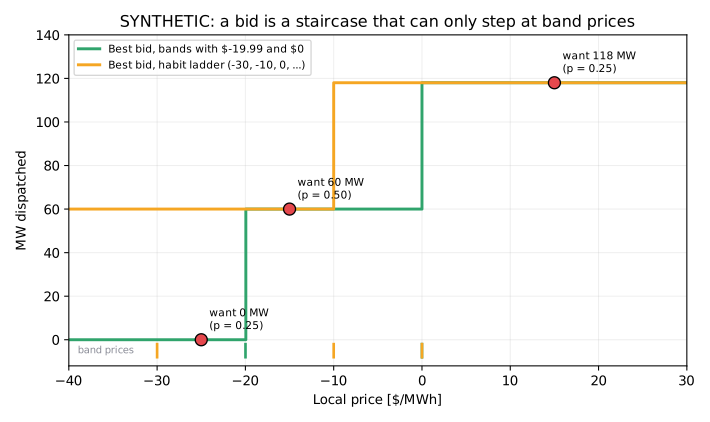
So a bid is a staircase: MW dispatched rises with the local price and can only step at a band price.
Two prices matter, and they differ:
- Local price: what dispatch is decided on. Behind a binding constraint it sits below the RRP: roughly the RRP minus the constraint's marginal value, times the unit's coefficient.
- RRP: what the unit is paid, adjusted by its loss factor. The PPAs in Chapter 6 are written on the RRP.
Price-setters are different
Behind a binding limit the farms' own bands often set the local price. Then what matters is not "the local price is X" but the order of the bands. That is the make-room case (§10). The cents matter there: −$19.98 sits behind −$19.99.
3 · The decision¶
- Intraday: MW per band, \(m_1, \dots, m_{10} \ge 0\), with \(\sum_i m_i = A\), the unit's available MW (for a semi-scheduled farm, its forecast availability).
- Day-ahead: which ten prices \(b_1 < \dots < b_{10}\) to offer, from a list of candidates.
4 · Variables and the four views¶
| View | What it sees |
|---|---|
| Physical | MW available; dispatch capped by availability and the network |
| Mathematical | a rising staircase \(D(P) = \sum_{b_i \le P} m_i\) |
| Optimiser | an LP in the band volumes; a MILP in the band prices |
| Economic | the value of each MW at each price; the value of each band price |
| Symbol | Meaning | Units |
|---|---|---|
| \(b_i\) | price of band \(i\) | $/MWh |
| \(m_i\) | MW in band \(i\) | MW |
| \(P_s\) | local price in scenario \(s\) | $/MWh |
| \(\pi_s\) | probability of scenario \(s\) | – |
| \(V_s(D)\) | value of dispatching \(D\) MW in scenario \(s\) | $/h |
5 · Objective¶
You know what you want at each local price, but not which price will happen. So you maximise the expected value of the staircase:
The simplest \(V_s\) is a target with penalties: "at −$15 I want 60 MW; each MW short costs $45/MWh, each MW over costs $25/MWh". Any concave piecewise-linear value works. That includes "each MW is worth what my contract pays, until the limit, and then less", which is how §10 values North's MW.
6 · Constraints¶
- Volumes: non-negative, and summing to the available MW.
- Prices: strictly increasing, whole cents, at most ten, and fixed for the day. The intraday problem treats them as data.
- Market rules: offers within the market floor and cap. Rebids need a verifiable reason recorded at the time, and offers must be made in good faith.
- Contracts and operating rules: South may not offer below −$19.99 (Chapter 6). Making room for another company's farm is a decision for both owners and their lenders (Chapter 7).
7 · Formulation¶
Why these techniques? Structure → method¶
| Property of the problem | Here | So |
|---|---|---|
| Two clocks | band volumes are continuous and rebid-able; band prices are fixed a day ahead | two models: an LP for volumes, a MILP for prices |
| Intraday objective | linear in the band volumes, once each scenario's value is split into concave pieces | an LP with no binaries: concavity fills the pieces in order |
| Constraints | one equality (\(\sum_i m_i = A\)), one equality per scenario linking bands to dispatch, and bounds | in textbook simplex the equalities need artificial variables; HiGHS handles them internally |
| Day-ahead decision | choose at most 10 prices from many candidates | a discrete choice: one binary per candidate price |
| Linking | \(m_{t,c} \le A_t\, y_c\) | a big-M row whose M is the physical bound \(A_t\), as tight as it can be |
| Size | scenarios × bands for the LP; intervals × candidates for the MILP | small enough for exact solution with HiGHS |
| Impossibility | a staircase cannot fall | some targets are infeasible for any bid; the LP finds the best hedge |
Chosen.
- An LP for band volumes. Given prices and scenarios, "which MW go where" is
linear. Its optimum is a vertex, and its duals price each scenario's constraint.
- A MILP for band prices. "At most ten prices" is a cardinality limit on yes/no
choices. Branch and bound searches the choices and proves how close it is to the
best.
- Gap detection (find_gaps) before any solve: sort scenarios by price and look for
neighbours that want different MW with no band between them.
Not chosen.
- Enumerating price sets. Choosing 10 from, say, 100 candidates has about
\(1.7 \times 10^{13}\) combinations. Branch and bound with an LP bound avoids it.
- A rule such as quantile bands (the Chapter 9 daily_bands rule). Cheap and
reasonable, and kept as the baseline; it cannot see that a price only matters when
it sits between a cliff and a break-even.
- Continuous relaxation of the binaries. It would spread each band across fractions
of many prices, which no bid can express.
- A bilevel or equilibrium model of the clearing. It needs the engine's full rules;
the dispatch rule here is our approximation, not NEMDE.
What the theory guarantees. - The LP is solved to a proven optimum, and the MILP returns a proven gap. Neither can beat a bid with unlimited bands. The "falling target" limit is a fact about staircases, not a solver weakness.
References. - Wolsey (2021), Integer Programming: tight big-M and indicator formulations (Chapter 5). - Land and Doig (1960), An automatic method of solving discrete programming problems: branch and bound (Choosing a technique). - Charnes (1952), Optimality and degeneracy in linear programming: the big-M penalty on artificial variables (same section). - Pinson, Chevallier and Kariniotakis (2007), and Morales, Conejo and Pérez-Ruiz (2010): bids as quantiles of a forecast, and as stochastic programmes (Chapter 8). - Choosing a technique for the LP-versus-MILP decision.
Intraday, an LP. Split each scenario's value into its concave pieces \(d_{s,k} \in [0, \ell_{s,k}]\), each worth \(g_{s,k}\) per MW, with \(g_{s,1} \ge g_{s,2} \ge \dots\):
Because the pieces are concave, the LP fills them in order without needing binaries.
What the bands can and can't do. Sort the scenarios by price. Two neighbouring scenarios can only get different MW if some band price lies between them. That gives two kinds of failure:
- A missing band: a gap between two prices that want different MW. Tomorrow's bands can fix it.
- A falling target: wanting fewer MW at a higher price. No bid can ever do this: a staircase only rises.
Day-ahead, a MILP. Add a binary \(y_c\) for each candidate price, and give every interval \(t\) its own volumes \(m_{t,c}\):
The objective is the sum over the day of each interval's expected value. Many candidate prices dispatch identically: any price between the same two scenario prices. So the solution is tidied afterwards: each chosen price moves to the economically meaningful point in its gap, and empty bands are dropped.
8 · Visualisation¶
The figure in §2 is the whole idea. The targets are the three red dots: 0 MW at −$25, 60 MW at −$15, all 118 MW at +$15. A set with a band at −$19.99 (green) builds a staircase through all three. The "habit" ladder (−30, −10, 0, …; orange) has nothing between −$25 and −$15, so those two prices must get the same MW. The LP gives 60 MW to both: −$25 is a quarter as likely as −$15.
9 · Implementation¶
from energy_or.bidding import ValueScenario, allocate_volumes, find_gaps
from energy_or.data.bands import HABIT_BANDS

targets = (  # local price, probability, MW wanted, available, $/MWh short, $/MWh over
    ValueScenario.from_target(-25.0, 0.25, 0.0, 118.0, 40.0, 30.0),
    ValueScenario.from_target(-15.0, 0.50, 60.0, 118.0, 45.0, 25.0),
    ValueScenario.from_target(15.0, 0.25, 118.0, 118.0, 55.0, 0.0),
)
bid = allocate_volumes(HABIT_BANDS, available_mw=118.0, scenarios=targets)
bid.volumes_mw  # 60 MW at −$1,000, 58 MW at −$10
bid.cost_of_bands  # $37.50 per interval lost to the missing band
find_gaps(HABIT_BANDS, targets)  # [BandGap(low_price=-25.0, high_price=-15.0, ...)]
| Artefact | Location |
|---|---|
| Staircase, allocation LP, gaps, band-design MILP, band values | src/energy_or/bidding/bands.py |
| Make-room bids behind a shared limit | src/energy_or/bidding/portfolio.py |
| Tomorrow's synthetic intervals, habit and designed band sets | src/energy_or/data/bands.py |
| Tests | tests/test_bands.py |
10 · Solve¶
"At this local price I want this many MW"¶
| Bands | MW per band | Dispatch at −$25 / −$15 / +$15 | Lost to the bands |
|---|---|---|---|
| −1000, −19.99, 0, 300 | 60 @ −19.99, 58 @ 0 | 0 / 60 / 118 | $0 |
| Habit ladder | 60 @ −1000, 58 @ −10 | 60 / 60 / 118 | $37.50 per interval |
The rule a trader can use without any solver: to get \(Y\) MW at local price \(P\), put \(Y\) MW in bands priced at or below \(P\) and the rest above it. It only fails when two prices you care about have no band between them.
Making room behind the shared limit¶
When the limit binds, North and South set the local price themselves, so the bid has to get the order right. South offers all its MW at −$19.99, its lowest permitted price. North's make-room decision becomes two numbers:
| Band | MW | Dispatched when | |
|---|---|---|---|
| Front | below −$19.99; best at North's break-even, −$64.99 | \(k\) | RRP ≥ band price, ahead of South |
| Behind | just above −$19.99: −$19.98 | \(A - k\) | only into room South leaves, or when the limit doesn't bind |
With North at 180 MW, South at 110 MW and a 200 MW limit, the λ-weighted value from Chapter 7 (South at 85 % of budget) chooses:
| Predispatch RRP (± $12) | Front MW at −$64.99 | Behind MW at −$19.98 |
|---|---|---|
| +$20, −$10, −$16 | 90 | 90 |
| −$20, −$30 | 180 | 0 |
The switch comes at a predispatch price of about −$16.75. Below that, there's too much chance the RRP lands under −$20. Then South doesn't clear, North's behind MW don't either, and the room is wasted. This is Chapter 6's cliff, now written as band volumes. With plain dollars (λ = 1 for both), North keeps all its MW in front at every price, which is Chapter 6's conclusion.
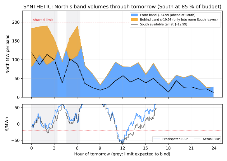
Through tomorrow, the limit is expected to bind in 65 of 288 intervals. North makes room in all 65 and keeps everything in the front band otherwise.
Can yesterday's habit ladder do it?¶
Mostly, yes. The habit ladder has −$50 below South (instead of −$64.99) and −$10 above it (instead of −$19.98). Over tomorrow it loses about $50 of λ-weighted value. That is small because the behind band's price only matters when the RRP lands between −$19.99 and it, and there is spare room under the limit.
What is each band price worth?¶
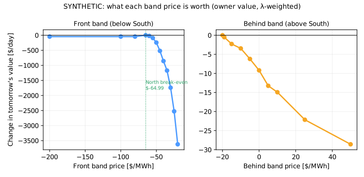
- The front band matters most. Every dollar it sits above North's break-even loses output whenever the RRP lands in between. At −$40 tomorrow loses about $860; at −$20, about $3,600. Below the break-even (−$100, −$1,000) the farm runs at a loss in deep negative prices, a small cost on this day.
- The behind band is cheap to get slightly wrong: $3 at −$10, $29 at +$50. But it must be above −$19.99, or North jumps the queue and the room is gone.
11 · Interpret¶
What to tell a trading desk
- A bid is a staircase. To get \(Y\) MW at local price \(P\), put \(Y\) MW at or below \(P\) and the rest above it. Bands only limit you where two prices you care about have nothing between them.
- No bid gives less MW at a higher price. If your plan needs that, the bid can only hedge it, and the LP finds the best hedge.
- Behind a binding limit, order beats level. Making room is "front MW at North's break-even, the rest one cent behind South". Have both prices in tomorrow's bands.
- Price your bands from your contracts: break-evens, cliffs and minimum offers first, then spare steps. On this portfolio the front band is worth hundreds to thousands of dollars a day; the other bands are worth tens.
12 · Backtest¶
Tomorrow's bids were chosen on predispatch with a $12 error and then settled at the actual RRP. A proper backtest would replay archived predispatch and the real bands the desk submitted, rebid by rebid, using only information available at the time (Milestone 7). Your own bid files (bid periods and band availabilities) would let the book measure how often the bands actually limited the desk.
13 · Adding realism¶
- Constraint coefficients and loss factors. Offers are referred to the regional node through the unit's loss factor. Check whether South's −$19.99 floor and its −$20 cliff are on the same basis: at a loss factor of 0.95, an offer of −$19.99 is about −$21 at the regional node.
- Other units behind the constraint. If others bid lower, the local price can sit far below the RRP while the RRP still pays. That is the incentive behind floor-price bidding when constrained (Part XIII).
- Ties. Two units at the same price behind a constraint are dispatched in proportion, which is why one cent decides the order.
- Rebid timing. Late rebids carry more scrutiny; volume shifts should be planned as predispatch updates, not at the last minute.
- More units, more bands. A battery uses all ten bands (charge and discharge at several prices). Its band design is where the MILP earns its keep.
14 · Exercises¶
Guided
Allocate the three targets by hand with bands −1000, −20, −10, 0, then check with
allocate_volumes. Which target is missed, and why?
Engineering
Write a rebid validator: refuse volumes that don't sum to the available MW, or a price that isn't one of today's bands, and log the reason with the inputs that justified it.
Market
South moves its offer to −$19.90. What must North's behind band be now, and what happens if yesterday's bands still say −$19.98?
Challenge
Choose North's ten band prices for a whole synthetic week with a MILP, given uncertain λs. How many bands does it actually use?
Production challenge
Design the rebid record: timestamp, interval, band volumes before and after, the predispatch and λs that drove it, and the reason text. What would an auditor need to reproduce the decision?
15 · Production perspective¶
- Two jobs, two schedules. A day-ahead job proposes band prices (MILP) for a human to approve before the deadline; an intraday job sets band volumes every predispatch run (LP or two-band search) and submits rebids within a latency budget.
- Guardrails. Never place North's behind band at or below South's price. Never rebid on stale predispatch. Check volumes against availability and the UIGF.
- Explain every rebid. Log what changed, why (the forecast and λs), and what each scenario would have dispatched, so the trader and the auditor see the same thing.
- Measure decision value. Track value lost to the bands (
cost_of_bands) and to the staircase (cost_of_staircase). If band cost is persistently high, tomorrow's prices are wrong.
Run it yourself¶
| Artefact | Location |
|---|---|
| Bands, allocation, design | src/energy_or/bidding/bands.py |
| Make-room bids | src/energy_or/bidding/portfolio.py |
| Synthetic tomorrow | src/energy_or/data/bands.py |
| Tests | tests/test_bands.py |
| Notebook | notebooks/08_ten_price_bands.ipynb |