T3 · Least squares and gradient descent

Intermediate Optimisation toolbox Reliability

In this chapter

• Fit a turbine power curve from SCADA as a least-squares problem, and solve it three direct ways: normal equations, QR and SVD
• See why the condition number decides whether those answers can be trusted, and how the choice of basis changes it by fifteen orders of magnitude
• Derive gradient descent's step-size rule, watch it diverge above \(2/L\), and compare it with momentum, Nesterov and Adam
• Replace squares by absolute values and get a robust fit that is an LP, then add a monotone constraint, and see which fit gets the lost-energy number right
• Meet the first non-convex problem in the book: a logistic curve with two equally good optima

Chapters 3 to 5 priced every stop by the energy the turbine would have produced. That number comes from a power curve: what the turbine makes at a given wind speed when nothing is wrong. Nobody hands you that curve. You fit it from SCADA data that also holds curtailment, stops and noise, and the way you fit it moves the lost-energy figure by more than 10 %. Fitting it is the cleanest possible introduction to unconstrained optimisation: one objective, a closed-form answer, and every iterative method in machine learning can be tested against it.

---

1 · The real-world problem

An O&M contract guarantees energy-based availability in the high 90s (Chapter 3). Every month the owner and the contractor agree how much energy was lost to stops, and the contractor pays liquidated damages on the shortfall. The lost energy is

\[ E_\text{lost} = \sum_{\text{stopped samples } n} \hat P(v_n)\,\Delta t , \]

where \(v_n\) is the wind speed while the turbine was stopped and \(\hat P\) is the fitted power curve. Bias \(\hat P\) low and the contractor underpays. Fit it so badly that it isn't monotone and it will be disputed. The site manager's question is simple: which curve, fitted how?

2 · The physical system

One 3.4 MW turbine with 60 days of synthetic 10-minute SCADA (8,640 samples, energy_or.data.scada). The data mimic the patterns of the reference farm. Each sample has a nacelle wind speed, an active power and a status that real SCADA rarely labels cleanly:

Status	Share	What the power looks like
normal	91.7 %	the curve plus turbulence and measurement noise
curtailed	4.1 %	capped at 40–70 % of rated for a few hours
stopped	4.2 %	≈ 0 kW whatever the wind

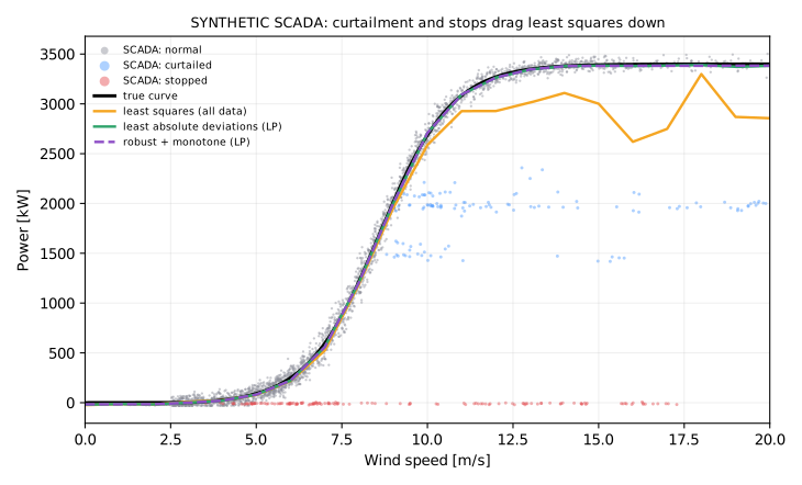
The grey cloud is the curve we want. The blue and red points are real operations that happen to look like bad data for this purpose.

3 · The decision

Choose the curve \(\hat P(v)\). Two decisions sit inside it: the shape family (the basis) and the loss (what counts as a good fit).

4 · Variables

Write the curve as a weighted sum of basis functions, \(\hat P(v) = \sum_k \beta_k \phi_k(v)\). The unknowns are the weights \(\beta\). Two bases:

• Hat functions on knots every 1 m/s from 0 to 20 m/s. \(\phi_k\) is 1 at knot \(k\), 0 at its neighbours and linear in between. So \(\beta_k\) is the power at knot \(k\) in kW and the curve is piecewise linear. This is how a manufacturer's power-curve table works.
• Polynomials, \(\phi_k(v) = v^k\), raw or scaled to \(v/25\).

Either way, stacking \(\phi_k(v_n)\) into a matrix \(X\) (\(n \times k\)) makes the fitted powers \(X\beta\). The model is linear in \(\beta\) even though the curve is not linear in \(v\).

5 · Objective

Ordinary least squares minimises the mean squared error,

\[ f(\beta) = \frac{1}{n}\,\lVert X\beta - y \rVert_2^2 . \]

It is smooth and convex, and its gradient is \(\nabla f = \tfrac{2}{n} X^\top(X\beta - y)\). Setting that to zero gives the normal equations:

\[ X^\top X\,\beta^\star = X^\top y . \]

Geometrically, \(X\beta^\star\) is the orthogonal projection of \(y\) onto the span of the columns of \(X\). The residual is perpendicular to every basis function.

Existence and uniqueness (T2, again)

A least-squares optimum always exists: the objective is bounded below by zero. It is unique exactly when \(X\) has full column rank. With 0.5 m/s knots and only 30 days of data, one knot can have no samples near it. Its column is then almost zero, \(X^\top X\) is singular, and any power at that knot fits equally well. The SVD returns the minimum-norm answer, which is a tie-break rule like T2's. Better still, don't place knots where there is no data. The book's knots stop at 20 m/s for this reason.

6 · Constraints (optional, and useful)

Unconstrained least squares will happily produce a curve that dips with wind speed. A real power curve is non-decreasing up to cut-out. Write the knot powers as cumulative increments, \(\beta_k = \sum_{j \le k} \delta_j\), with \(\delta_j \ge 0\) for \(j \ge 1\). The problem becomes bounded least squares (scipy.optimize.lsq_linear) or, with absolute errors, an LP. It is still convex, and monotonicity is guaranteed instead of hoped for.

7 · Formulation: one problem, four losses

Fit	Objective	Problem class	Solver
OLS	\(\sum_n r_n^2\)	unconstrained QP, closed form	QR / SVD
LAD	\(\sum_n \lvert r_n\rvert\)	LP	HiGHS
Huber	\(\sum_n h_\delta(r_n)\)	smooth convex	IRLS
Monotone LAD	\(\sum_n \lvert r_n\rvert\), \(\delta \ge 0\)	LP	HiGHS

Here \(r_n = (X\beta)_n - y_n\). Least absolute deviations is an LP once each residual is split into its positive and negative parts:

\[ \min_{\beta,\,u,\,w} \ \sum_n (u_n + w_n) \quad\text{s.t.}\quad X\beta - y = u - w,\qquad u, w \ge 0 . \]

At the optimum at most one of \(u_n, w_n\) is positive, so \(u_n + w_n = \lvert r_n \rvert\). LAD fits the conditional median instead of the mean. With one constant and data \((1, 2, 3, 4, 100)\), least squares answers 22 and LAD answers 3 (a test in tests/test_curve_fit.py). Huber's loss is quadratic for \(\lvert r\rvert \le \delta\) and linear beyond, so it behaves like OLS for noise and like LAD for outliers.

8 · Visualisation

The figure in §2 tells the story. Least squares (orange) is dragged down above 10 m/s, where curtailed and stopped samples pull on the mean. At 15 m/s it says 3,002 kW against a true 3,400 kW. LAD (green) and monotone LAD (purple) sit on the true curve, because a median doesn't care how far the bad points are, only that they are a minority.

Why these techniques? Structure → method

Property of the problem	Here	So
Model	a power curve that is linear in its knot powers: \(y \approx X\beta\)	least squares: convex, with an optimum that always exists
Uniqueness	unique exactly when \(X\) has full column rank	choose knots where there is data
Conditioning	\(\kappa(X)\) is 67 for hat functions and \(1.5\times10^{13}\) for raw degree-9 monomials	QR by default, SVD when near rank-deficient, normal equations only if well conditioned
Contamination	8 % of samples are stops or curtailment, far from the curve	a loss that tolerates outliers: LAD (an LP) or Huber (IRLS)
Shape constraint	the curve should not fall with wind speed	\(\delta \ge 0\) increments: monotone LAD is still an LP
Iteration	a closed form exists	gradient methods are shown as the template where none does, and are checked against it
Nonlinear parameters	a logistic curve has a symmetry and is not convex	local solvers (Levenberg–Marquardt), as an entry to T4

Chosen. - QR and SVD because forming \(X^\top X\) squares the condition number, so it loses \(\log_{10}\kappa(X)^2\) of about 16 digits. QR works on \(X\) directly. SVD reports \(\kappa\) and drops negligible directions. - A well-conditioned basis, which matters more than the solver. Hat functions are local, so they overlap only their neighbours. - LAD as an LP because the loss is a modelling decision. Least squares fits the mean and understates lost energy by 11 %. LAD fits the median and gets within 0.5 % without being told which samples are bad. - Nesterov and heavy ball because on a quadratic they need about \(\sqrt\kappa\) iterations per digit instead of \(\kappa\), as the table of iteration counts shows.

Not chosen. - Normal equations on a poor basis. On raw degree-12 monomials they already fit worse than QR. - Adam or plain gradient descent as the solver. Adam rescales each coordinate and is no cure for conditioning. On the polynomial basis it needed 305,051 iterations against 29,286 for Nesterov. - Dropping samples by status flag. It is the most accurate here, but in real SCADA the flags often cannot be trusted. - Monotone constraints alone. They do not fix a biased loss. Monotone OLS is still 10 % low.

What the theory guarantees. - Least squares has a solution, and it is unique under full column rank. The error in \(\beta\) is amplified by at most about \(\kappa(X)\) for QR, and by \(\kappa(X)^2\) for the normal equations. - Gradient descent on a quadratic converges for every starting point if and only if \(\eta < 2/L\), at rate \(1 - 1/\kappa\) per step with \(\eta = 1/L\). - LAD is an LP, so the optimum is global, but it need not be unique. The logistic fit has no such guarantee.

References. - Golub and Van Loan (2013), Matrix Computations: QR, SVD and the normal equations. - Higham (2002), Accuracy and Stability of Numerical Algorithms: conditioning in floating point. - Nocedal and Wright (2006), Numerical Optimization: step sizes and convergence rates. - Polyak (1964) and Nesterov (1983): heavy ball and accelerated gradient. - Huber (1964) and Koenker and Bassett (1978): robust loss and LAD as an LP.

Full entries are in Further reading, T3. See also Choosing a technique.

9 · Implementation

import numpy as np

from energy_or.data.scada import turbine_scada
from energy_or.toolbox.curve_fit import hat_basis, lad_fit, lstsq, monotone_lad_fit

d = turbine_scada()  # SYNTHETIC
knots = np.arange(0.0, 21.0, 1.0)
X = hat_basis(d.wind_ms, knots)

ols = lstsq(X, d.power_kw, method="qr")  # kW at each knot
lad = lad_fit(X, d.power_kw)  # an LP in HiGHS
mono = monotone_lad_fit(d.wind_ms, d.power_kw, knots)  # LP with δ ≥ 0

Three direct solvers and the condition number

lstsq solves the same problem three ways:

• Normal equations: form \(X^\top X\) (\(k \times k\)) and solve it. This is the fastest (0.5 ms here) but it squares the condition number.
• QR: \(X = QR\), then solve \(R\beta = Q^\top y\). It works on \(X\) itself, so its error grows with \(\kappa(X)\), not \(\kappa(X)^2\).
• SVD: \(X = U\Sigma V^\top\). It is the most robust, it reports \(\kappa\) directly, and it drops directions whose singular value is negligible.

The condition number \(\kappa(X) = \sigma_\text{max}/\sigma_\text{min}\) bounds how much relative error in the data (or in floating-point rounding) can be amplified in \(\beta\). Double precision carries about 16 digits. Normal equations lose \(\log_{10}\kappa(X)^2\) of them.

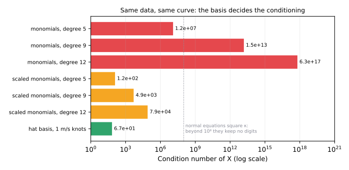
The curve, data and objective are the same in every row; only the basis changes. Raw monomials of degree 9 have \(\kappa \approx 1.5\times10^{13}\): squared, that is beyond what double precision can represent. Scaling wind to \(v/25\) buys ten orders of magnitude. The hat basis has \(\kappa \approx 67\) because each column is local: it only overlaps its neighbours. Choosing a well-conditioned parametrisation is the single most effective numerical decision in least squares. On raw degree-12 monomials the normal equations already find a worse fit than QR (MSE 235,619 against 234,814 kW²), even though both are "the" least-squares solution. SVD's default tolerance deliberately throws away the near-null directions there (MSE 243,296). That is a slightly worse fit with tamer coefficients, which is regularisation by truncation.

10 · Solve: gradient descent and its relatives

The closed form exists, so why iterate? Because almost nothing else in optimisation has one: neural forecasters, nonlinear models, problems with millions of variables. Least squares is where you can check an iterative method against the exact answer.

The step-size rule, derived

The Hessian of \(f\) is constant: \(H = \tfrac{2}{n}X^\top X\), with eigenvalues between \(\mu\) (smallest) and \(L\) (largest). For a quadratic, the error \(e_t = \beta_t - \beta^\star\) of gradient descent with step \(\eta\) obeys

\[ e_{t+1} = (I - \eta H)\, e_t . \]

Each eigen-direction shrinks by \(\lvert 1 - \eta\lambda\rvert\) per step. That is below 1 for every \(\lambda\) if and only if \(\eta < 2/L\). With the safe choice \(\eta = 1/L\), the slowest direction shrinks by \(1 - \mu/L = 1 - 1/\kappa\) per iteration, where \(\kappa = L/\mu = \kappa(X)^2\). That is about \(2.3\,\kappa\) iterations per digit of accuracy.

The test suite checks this on \(X = \operatorname{diag}(1, 3)\), where \(L = 9\). Step \(1.9/L\) converges and \(2.1/L\) diverges, exactly as derived.

Acceleration

• Heavy ball (Polyak momentum) adds a fraction \(\beta\) of the previous step. Tuned for a quadratic (\(\eta = 4/(\sqrt L + \sqrt\mu)^2\), \(\beta = \big(\tfrac{\sqrt\kappa - 1}{\sqrt\kappa + 1}\big)^2\)), it needs about \(\sqrt\kappa\) iterations per digit instead of \(\kappa\).
• Nesterov evaluates the gradient at the look-ahead point \(\beta_t + \beta v_t\). It has the same \(\sqrt\kappa\) rate and is better behaved early on.
• Adam divides each coordinate's step by a running RMS of its gradient: a cheap, diagonal rescaling. It is the default for training neural networks, not a conditioning cure.

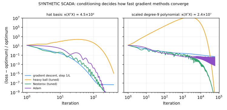
Iterations to reach a loss within \(10^{-6}\) (relative) of the optimum:

Method	Hat basis, \(\kappa(X^\top X) \approx 4.5\times10^3\)	Scaled degree-9 polynomial, \(\kappa \approx 2.4\times10^7\)
Gradient descent, \(\eta = 1/L\)	93	not converged after 400,000 (gap 3.5 %)
Heavy ball (tuned)	447	47,031
Nesterov (tuned)	116	29,286
Adam	151	305,051
QR (direct)	one factorisation	one factorisation

Three things to see:

1. Conditioning is the whole story. The same methods, data and curve need roughly 100 times more iterations when the basis is badly conditioned. On the polynomial, \(\sqrt\kappa \approx 4{,}900\) against \(\kappa \approx 2.4\times10^7\) is why acceleration wins.
2. The loss converges before the parameters do. On the hat basis, gradient descent reaches the loss target in 93 iterations, far fewer than \(2.3\kappa\) per digit predicts. The loss gap weighs each direction by its eigenvalue, so the slow directions hardly show. Those directions are knots with almost no data. After 93 iterations, the power at 0 m/s (one nearby sample) is still 23 kW off, and the powers at 17–18 m/s are 4–5 kW off. That is the flat tail in the left panel. A converged loss does not mean converged coefficients. Check the parameters you will use.
3. Momentum isn't monotone. The tuned heavy ball's loss first rises, by a factor of 18 on the hat basis and a million on the polynomial, before it falls faster than anything else. It is a transient from the momentum term, not divergence. A stopping rule that kills a run when the loss rises would wrongly kill it.

11 · Interpret: the lost-energy number

The decision value is the lost energy that each curve assigns to the 363 stopped samples:

Curve	Power at 15 m/s	RMSE vs true curve, 3–18 m/s	Lost energy	Bias
True curve (synthetic truth)	3,400 kW	0	101.9 MWh	—
OLS, all data	3,002 kW	312 kW	90.7 MWh	−11.1 %
OLS, monotone	2,973 kW	271 kW	91.6 MWh	−10.1 %
Huber, \(\delta = 100\) kW	3,382 kW	18 kW	101.1 MWh	−0.8 %
LAD (LP)	3,385 kW	12 kW	101.4 MWh	−0.5 %
Monotone LAD (LP)	3,382 kW	12 kW	101.4 MWh	−0.5 %
OLS, normal samples only	3,396 kW	7 kW	101.9 MWh	0.0 %

The lesson

The loss function is a modelling decision, not a numerical detail. With 8 % of the samples contaminated, least squares understates lost energy by 11 %. In an availability-guarantee calculation, that is 11 % of the damages the contractor owes. The LP (LAD) gets within 0.5 % without being told which samples are bad. A monotone constraint does not fix a biased loss: monotone OLS is still 10 % low. Filtering by status is best of all, but only when the status flags can be trusted, and in real SCADA they often can't.

12 · Backtest

The synthetic truth is a luxury. With real SCADA you validate out of sample. Fit on days 1–30, then score on the normal samples of days 31–60:

Fit	Hold-out RMSE on normal samples	Lost-energy bias, days 31–60
OLS, 1 m/s knots	219 kW	−0.4 %
LAD, 1 m/s knots	63 kW (≈ the noise level)	−0.6 %
LAD, 2 m/s knots	71 kW	+1.9 %

Robustness holds up out of sample. The lost-energy bias of OLS nearly disappears in the second month, though. Its stops happened at low wind (10.8 MWh lost in total), where contamination barely bends the curve. The value of a better curve depends on when the turbine stops. It is largest when stops coincide with high wind, which is exactly when lost energy matters most. Coarser knots add bias where the curve bends fastest.

13 · Adding realism

• Air density. IEC 61400-12 normalises wind speed to a reference density. Winter and summer curves differ by a few per cent.
• Nonlinear models. A four-parameter logistic \(\hat P(v) = a + \frac{r - a}{1 + e^{-(v - v_0)/s}}\) is nonlinear in its parameters. Levenberg–Marquardt (scipy.optimize.least_squares) fits it to the normal samples: \(r = 3{,}400\) kW, \(v_0 = 8.60\) m/s, \(s = 1.05\), RMSE 66 kW. Starting from \(s = -1\) instead gives \(a = 3{,}400\), \(r = -16\), \(s = -1.05\): a different parameter vector with exactly the same curve and the same loss. Swapping \(a \leftrightarrow r\) and negating \(s\) leaves the function unchanged. That symmetry means two separate global optima with a ridge between them, so the objective cannot be convex. It is the first non-convex problem in the book, and T4 takes it from here.
• Turbulence and hysteresis. Real scatter widens on the steep part of the curve, and the synthetic data model this. Weighted least squares can down-weight those samples.
• Degradation. Fit monthly and watch the knot powers drift. A falling rated plateau is a blade or pitch problem showing up in the data (Chapter 3's pitch faults).

14 · Exercises

Guided

For \(X = \operatorname{diag}(1, 3)\) and \(y = (1, 1)\), compute \(L\), \(\mu\) and \(\kappa\) by hand. How many gradient-descent iterations with \(\eta = 1/L\) does it take to shrink the error by \(10^{-6}\)?

Engineering

Add a check to the curve-fitting job that fails when \(\kappa(X) > 10^6\), when any knot has fewer than 20 samples, or when the fitted curve is not monotone. Which of these does the 0.5 m/s knot grid trip?

Market

The contractor proposes OLS on all data "because it is standard". At $80/MWh and this turbine's stops, what is the difference in monthly lost-energy value between their curve and the monotone LAD curve? Across 28 turbines?

Challenge

Show that Huber regression is the limit of LAD as \(\delta \to 0\) and of OLS as \(\delta \to \infty\), then write Huber as a convex QP with auxiliary variables.

Production challenge

A monthly job refits 28 curves with gradient descent and an early-stopping rule "stop if the loss rises twice in a row". It silently returns bad curves for some turbines. Using §10, explain which method and which turbines are most likely affected, and what the job should log.

15 · Production perspective

• Use a direct solver whenever one exists. QR on a 20-column problem is one factorisation. Gradient descent is for problems without a closed form.
• Log the condition number with every fit, the way OptOps logs solver status and gap. A jump in \(\kappa\) means a knot lost its data.
• Validate parameters, not just loss. The coefficients you publish (kW at each knot) are what the lost-energy calculation uses.
• Prefer robust losses on operational data. Status flags lag, curtailment is under-recorded, and an LP solves 8,640 samples in a fraction of a second.
• Version the curve. A lost-energy claim must be reproducible from the curve version, the data snapshot and the fitting code.

Run it yourself

Artefact	Location
Bases, direct and gradient solvers, robust and monotone fits, logistic NLS	src/energy_or/toolbox/curve_fit.py
Synthetic SCADA	src/energy_or/data/scada.py
Tests	tests/test_curve_fit.py
Notebook	notebooks/t3_least_squares_gradient_descent.ipynb