12 · Two contracts, one line: who should use it, hour by hour¶

Intermediate Advanced Case H · Case L LP duality · parametric LP · game theory

In this chapter

Two neighbouring wind farms of the fictional Lantern Bay portfolio share one 250 MW line. Same wind, different contracts: a contract for difference suspended at negative prices, and an as-produced PPA
Derive what one more MWh is worth to each owner, and find that priority switches at $32/MWh
Solve the year five ways:
- a closed form, hour by hour
- one LP with the line's shadow price every hour
- a parametric LP that values a bigger line
- the market's price-ordered clearing
- coordinated rebids from an hour-ahead forecast
If the farms belonged to different owners, split the gain fairly with the Shapley value, and price the side payment per MWh

Chapter 6 asked how two farms behind one limit should bid, over a week, with one farm's contract dominating. Here the same question is asked over a year of a portfolio built from public project archetypes, where neither contract dominates. The answer depends on the price, so the methods change: duals priced hour by hour, a parametric LP for the line itself, and a cooperative game for the owners.

1 · The real-world problem¶

Two wind farms share a new 132 kV line to the transmission network:

Saltbush Plains Wind, 210 MW, sells 75 % of its output through a state-backed contract for difference. It receives strike − price on each MWh, at a $72 strike; the contract is suspended when the price is negative, and the state takes the certificates for that share.
Quandong Ridge Wind, 100 MW, sells 95 % of its output as produced to a data-centre owner at $68, certificates included.

Together they can produce 310 MW, but the line carries 250 MW. In 2,118 hours of the synthetic year (24 %), the wind is strong enough that someone must be curtailed. Who?

2 · The physical and market system¶

The line is a radial export limit: whatever the two farms send cannot exceed 250 MW. The market dispatches offers in price order behind the limit, cheapest first, and splits ties pro rata (a simplified stand-in for the network constraint in dispatch; not NEMDE). Both farms see the same regional price and have the same loss factor (0.94). The data are one synthetic hourly year (energy_or.data.portfolio).

3 · The decision¶

Each hour: how many MW each farm sends down the line. In the market, the decision is made through offers: the price at which each farm is willing to be dispatched.

4 · From contract to value per MWh¶

What one more MWh is worth to its owner, at regional price $p$:

\[ v_S(p) = 0.94\,p + \underbrace{0.75\,(72 - p)\,\mathbb 1\{p \ge 0\}}_{\text{CfD, suspended below } \$0} + \underbrace{0.25 \times 30}_{\text{own certificates}}, \qquad v_Q(p) = 0.95 \times 68 + 0.05\,(0.94\,p + 30). \]

So for $p \ge 0$, $v_S = 61.5 + 0.19\,p$ and $v_Q = 66.1 + 0.047\,p$. They cross at

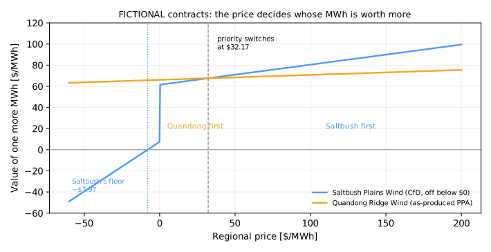
\[ p^\ast = \frac{66.1 - 61.5}{0.19 - 0.047} \approx \$32.17/\text{MWh}. \]

Value of one more MWh against the regional price

Below Saltbush's floor (−$7.97). Saltbush loses money on every MWh: its CfD pays nothing, and the price is negative. Quandong, mostly paid a fixed $68, would run down to the market floor. Quandong first; Saltbush off.
From −$7.97 to $32. Both want to run, but Quandong's MWh is worth more: its fixed price beats Saltbush's CfD top-up plus a small merchant share. Quandong first.
Above $32. Saltbush keeps 25 % of a rising price (plus certificates), while Quandong's revenue barely moves. Saltbush first.

The library computes these values from the contract terms and checks them against the settlement code's finite difference (agreement to 10⁻¹⁰).

5 · Objective¶

Maximise the portfolio's value over the year:

\[ \max_{d} \ \sum_t \big( v_S(p_t)\,d_{S,t} + v_Q(p_t)\,d_{Q,t} \big). \]

6 · Constraints¶

\[ d_{S,t} + d_{Q,t} \le 250, \qquad 0 \le d_{i,t} \le a_{i,t} \quad \text{(available wind)}. \]

7 · Formulation: five ways to answer¶

Why these techniques? Structure → method¶

Property of the problem	Here	So
Objective	linear in each farm's MW, with a value per MWh from its contract	an LP; the contract cliffs sit in the value, not in the model
Variables	two continuous MW per hour, 17,520 in the year	no integers
Constraints	one line row per hour, both coefficients 1, plus availability bounds	each hour is a one-row knapsack, so the closed form (rank by value, fill the line) is exact
Time coupling	none: no storage, so hours are independent	the year LP is block-diagonal; it is solved for its duals, not its answer
Question about the line	what is one more MW of limit worth, and how does that change with the limit?	parametric LP: re-solve over the limit, read the slope
Who decides	the market clears by offers; a forecast drives the rebids	a rule from the ranking, tested against hindsight
Two owners	the coordinated plan helps one and costs the other	cooperative game: a split that both prefer to acting alone

Chosen. - Closed form and year LP together. They agree to the cent; the LP is kept because its duals on the hourly line rows are the line's hourly shadow prices. - Parametric LP over the limit. Its value is a concave, piecewise-linear function of the limit, so the slope is the value of one more MW and it falls as the line grows. This is the number a connection negotiation needs. - Shapley value and the core for the payment. Each farm receives what it earns alone plus half the joint gain, and neither can do better by leaving.

Not chosen. - A MILP. There is no on/off decision once the contract values are per MWh. - A stochastic programme for the rebids. The decision is a threshold on the forecast ranking. The noise sweep measures its decision value directly, and shows when to stop coordinating. - The nucleolus or Nash bargaining. With two players they give the same split as Shapley, so the choice matters only when the fleet has three or more farms. - Finite differences on the dispatch. They need many solves and are unstable at degenerate points; the dual is exact where it is unique (see T2).

What the theory guarantees. - Ranking by value is optimal for each hour's one-row LP, and the value is concave in the limit. With two players and a positive joint gain, the Shapley split lies in the core. Where the optimum is degenerate (equal values), the dual is a range, not a number.

References. - Shapley (1953), A value for n-person games, and Shapley and Shubik (1954): the axioms behind the split (Chapter 12). - Peleg and Sudhölter (2007), Introduction to the Theory of Cooperative Games: the core, nucleolus and Shapley value together (Chapter 12). - Simshauser (2021), Renewable energy zones in Australia's NEM: shared-network curtailment in practice (Chapter 12). - Choosing a technique for when duals are worth a full LP.

Technique	What it gives	Where
Closed form, hour by hour: rank by value, fill the line, never run a negative-value MWh	The optimum	`optimal_dispatch`
One LP for the year (17,520 variables, 8,760 line rows)	The same optimum and the line's hourly shadow price	`optimal_dispatch_lp`
Parametric LP over the line limit	Value of the portfolio, and of one more MW of line, against limit	`line_value_curve`
Market clearing of offers at each farm's own floor	What happens if each farm bids for itself	`clear_with_floors`
Coordinated rebids from an hour-ahead forecast	What the portfolio can capture in practice	`coordinated_rebids`

The closed form and the LP agree to the cent, as they must: for a single coupling row per hour, ranking by value is the LP optimum. The LP earns its place through its duals.

8 · Visualisation: who is curtailed, and what the line is worth¶

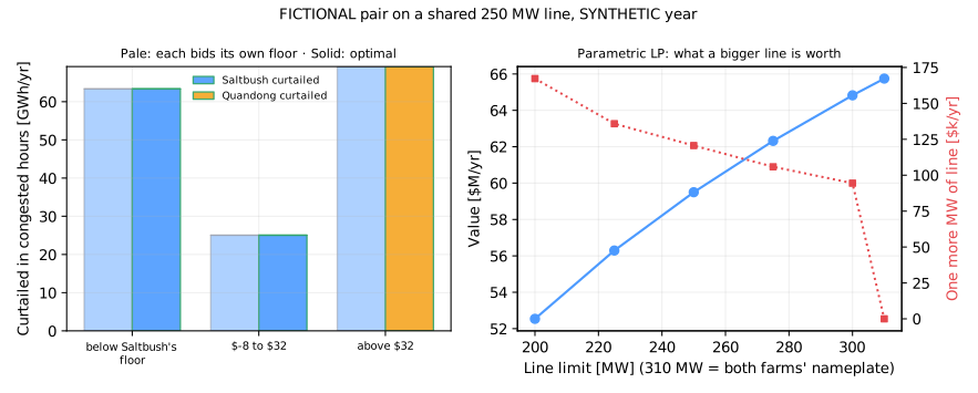
Curtailment by price band, and the value of a bigger line

The 2,118 congested hours fall into the three price bands:

Congested hours	Count	Own-floor bidding curtails	Optimum curtails
Price below −$7.97	304	Saltbush (it switches off)	Saltbush
−$7.97 to $32.17	470	Saltbush	Saltbush
Above $32.17	1,344	Saltbush	Quandong

All of the value at stake sits in the top band. When the price is high, the line should carry Saltbush's MWh, but Quandong's offer at the market floor puts it first.

9 · Implementation¶

from energy_or.contracts.shared_line import (
    clear_with_floors,
    coordinated_rebids,
    hour_ahead_forecast,
    line_case,
    optimal_dispatch_lp,
    sharing_agreement,
)
from energy_or.data.portfolio import portfolio_year

case = line_case(portfolio_year(), limit_mw=250)  # FICTIONAL, SYNTHETIC
best = optimal_dispatch_lp(case)  # optimum + hourly line shadow price
own = clear_with_floors(case)  # each farm bids its own floor
coord = coordinated_rebids(case, hour_ahead_forecast(case.price_per_mwh))
deal = sharing_agreement(case, own, coord)

10 · Solve: the line's shadow price, and sizing the line¶

The LP's dual on hour $t$'s line row, $\pi_t$, is what one more MW of line is worth that hour. Summed over the year, it is the value of one more MW of line capacity. Re-solving at different limits gives the parametric curve:

Line limit	Portfolio value	One more MW of line is worth	Congested hours
200 MW	$52.54M	$167k/yr	2,686
225 MW	$56.29M	$136k/yr	2,374
250 MW	$59.50M	$121k/yr	2,118
275 MW	$62.32M	$106k/yr	1,887
300 MW	$64.83M	$94k/yr	1,695
310 MW (nameplate)	$65.75M	$0	0

The curve is concave: each extra MW relieves fewer, cheaper hours. This is the number a connection negotiation needs. A 25 MW upgrade, from 250 to 275 MW, is worth $2.8M a year to this portfolio. Compare that with its cost, and with what the network operator would charge.

11 · Interpret: the market, coordination, and two owners¶

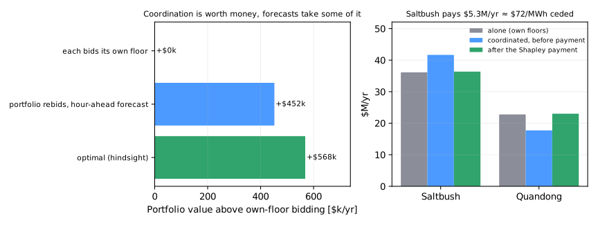
Policies compared, and the fair split between owners

Policy	Saltbush	Quandong	Portfolio	vs own floors
Each farm bids its own floor	$36.14M	$22.79M	$58.93M	—
Portfolio rebids on an hour-ahead forecast	$41.66M	$17.72M	$59.38M	+$452k
Optimal (hindsight)	$41.57M	$17.93M	$59.50M	+$568k

Bidding your own floor is not enough. Each farm's floor is right for itself. But Quandong's floor is the market floor, so it always goes first, including in the 1,344 hours when Saltbush's MWh is worth more.
Coordination needs only a rebid. When the forecast says Saltbush is worth more and the line will bind, Saltbush offers at the market floor and Quandong one cent behind it: Chapter 8's make-room trick. Otherwise both offer their own floors. With perfect price forecasts this reproduces the optimum exactly (a tested property).
The forecast costs 20 %. With a forecast that is $40/MWh off on average, it still captures $452k of the $568k.
A bad forecast is worse than none. The notebook sweeps the forecast noise. With more noise, coordination captures only 27 % of the gain, and with more still it does worse than each farm bidding its own floor. Each wrong call puts the less valuable farm first, or puts Saltbush at the market floor in an hour it should have been off. Judge a forecast by the decisions it drives, not by its error: coordinate only when the forecast is good enough to beat the do-nothing policy in a backtest.

One cent near the floor

Writing this chapter exposed a bug in the book's clearing function. It treated offers as tied using a relative tolerance, so −$1,000 and −$999.99 were "equal" and split pro rata, and the make-room trick silently failed at the market floor. Ties are now exact to a millionth of a dollar, a regression test guards it, and the earlier chapters' figures are unchanged. Floating-point tolerance is a modelling decision.

If the farms had different owners¶

Suppose each farm sat in its own project company, with different lenders. Then the coordinated plan costs Quandong $5.1M a year while Saltbush gains $5.5M, and Quandong's owner would refuse it. A line-sharing agreement fixes that with a side payment:

Shapley value. With two players, each gets what it earns alone plus half the joint gain: Saltbush $36.36M, Quandong $23.02M. Both are better off than alone, so the split is in the core.
The payment. Saltbush pays Quandong $5.3M a year. Spread over the MWh that move between the two farms, that is about $72 per MWh. It is close to the contract values themselves, because the payment mostly returns the value Quandong gives up (≈ $68–70 for each MWh it cedes); only a small part is Quandong's half of the $452k gain.

A per-MWh compensation price makes the deal operational: meter the MWh ceded in each coordinated hour, and settle monthly.

12 · Backtest¶

The coordinated policy decides each hour from a forecast that uses only the previous hour and the same hour yesterday (historical_only; a test changes the future and checks the forecast doesn't move). It is scored at actual prices. The gap to hindsight, $116k a year, is the honest cost of not knowing the price.

13 · Adding realism¶

5-minute dispatch and real offers. Ten bands set the day before, volumes rebid (Chapter 8). The coordinated rule needs only two bands per farm: the market floor and its own floor.
Constraint equations, not a radial line. In real dispatch, network constraints have coefficients on many units, and local prices can fall far below the regional price.
Contract details. Real contracts for difference may pay on a reference node, cap the difference payments, or count curtailed energy as "deemed" generation. Any of these changes $v_S$, and the method carries over unchanged.
Certificates are worth less in some years; the floor moves with them.

14 · Exercises¶

Guided

Re-derive $p^\ast$ if the CfD covered 60 % of output instead of 75 %. Which farm gains priority in more hours?

Engineering

Turn coordinated_rebids into a 5-minute rebid service: inputs are the forecast and both farms' availability; output is two offers per farm. What happens when the forecast is late?

Market

If the CfD paid strike − price even at negative prices, what are the new floor and crossover? Does the coordination value rise or fall?

Challenge

With three farms on the line, compute the Shapley value (six orderings) and show whether it is in the core for this year.

Production challenge

Write the monthly settlement report for the line-sharing agreement: MWh ceded, compensation paid, and an audit trail that shows each coordinated hour's forecast.

15 · Production perspective¶

Contract values are data. Keep value_per_mwh versioned alongside the contracts, and recompute floors when certificate prices or contract terms change.
Log the decision rule's inputs every hour: forecast, values, which farm was given priority. An owner will ask.
The line's shadow price is a KPI. Publish it monthly; it is the argument for, or against, an upgrade.

Run it yourself¶

Artefact	Location
Values, floors, crossover, LP, parametric LP, clearing, rebids, sharing	`src/energy_or/contracts/shared_line.py`
The fictional portfolio	`src/energy_or/data/portfolio.py`
Tests	`tests/test_shared_line.py`
Notebook	`notebooks/12_two_contracts_one_line.ipynb`