T1 · One model, many solvers
Intermediate Optimisation toolbox Case A

In this chapter
- Separate the model (what you want) from the solver (how it is found), and build Chapter 1's problem in SciPy, Pyomo and OR-Tools
- Solve it with HiGHS, GLOP, CLP, PDLP, CBC and SCIP, with Gurobi and CPLEX as drop-in backends when licensed, and check they agree
- Learn what differs: duals, tolerances, MIP gaps, model-building time, and which solvers can't do integers at all
- Meet a real engineering hazard: two packages that bundle different versions of the same solver can't live in one Python process
Chapter 1 solved Case A, two wind farms behind a 100 MW connection, with one tool. In a job you will meet a codebase in Pyomo, a colleague who swears by OR-Tools, and a licence for Gurobi. Can you move a model between them, and do you know what changes when you do? This chapter puts the same problem through every stack and compares the answers.
1 · The problem, once more
Two farms behind one shared limit, every five-minute interval of a day (or a week, a month, a quarter):
WF_A is merchant (spot plus certificates), WF_B holds a $65/MWh PPA, and the data is Chapter 1's synthetic day. One day is 576 variables and 288 constraints.
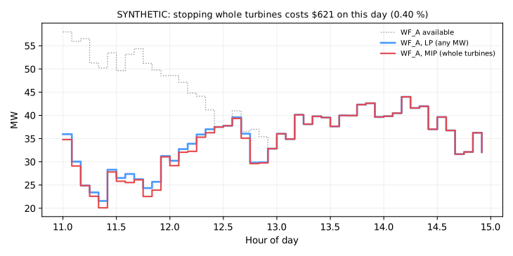
A MIP variant. A farm doesn't curtail by dialling to any MW: the controller stops whole turbines. With 25 turbines and all of them seeing the same wind, \(P_{ti} = (A_{ti}/25)\, n_{ti}\) with \(n_{ti} \in \{0,\dots,25\}\). Same objective, same limit, now with integers.
2 · Model versus solver
| Layer | What it is | Examples |
|---|---|---|
| Modelling layer | How you write the problem: variables, objective, constraints | SciPy matrices, Pyomo, OR-Tools pywraplp, PuLP, CVXPY, JuMP, AMPL, GAMS |
| Solver | The algorithm that finds the optimum | HiGHS, GLOP, CLP, PDLP (LP); HiGHS, CBC, SCIP, Gurobi, CPLEX (MIP) |
| Algorithm | Inside the solver | primal/dual simplex, interior point (barrier), first-order (PDLP), branch and bound |
A modelling layer that talks to many solvers lets you swap the engine without rewriting the model. Each does it differently:
- SciPy: you build the matrices yourself. It is fastest to build and the most error-prone.
- Pyomo: algebraic, readable, solver-independent. Building the model has a cost.
- OR-Tools: one API in front of many engines, including Google's own GLOP, PDLP and CP-SAT.
3 · The decision this chapter answers
Which modelling layer and solver should this problem use, and how would you know if two of them disagreed?
4 · Variables and the four views
| View | What it sees |
|---|---|
| Physical | MW per farm per interval, a 100 MW connection |
| Mathematical | an LP with 2 variables and 1 coupling row per interval (and an MIP twin) |
| Optimiser | build time, solve time, status, duals, gap |
| Economic | dollars over the horizon; value lost to whole-turbine steps |
Why these techniques? Structure → method
This chapter's question is which tool fits, so the table asks what the structure of the model implies for the solver, not only for the formulation.
| Property of the problem | Here | So |
|---|---|---|
| Objective | linear: value × MW × \(\Delta t\) | a linear programme (LP), which any LP solver accepts |
| Variables | 576 continuous for one day (17,280 for 30 days); the MIP twin adds integers \(n_{ti} \in \{0,\dots,25\}\) | too many to draw: an algebraic method (simplex, interior point or first-order) is required. Integers need branch and bound, so GLOP, CLP and PDLP cannot solve the twin |
| Constraint types | 288 rows of the form \(\le\), plus bounds | each \(\le\) row gets a slack variable; because \(P = 0\) is feasible, the simplex method starts at the origin and needs no artificial variables or big-M. A model with \(\ge\) or \(=\) rows would |
| Duals needed | the shadow price of the shared limit per interval | simplex or barrier with crossover returns them reliably; a first-order method (PDLP) returns them only to its tolerance; a MIP interface returns none |
| Structure | 288 independent rows, each coupling two farms | no time coupling, so very easy for every solver; differences are in building and in interface, not in difficulty |
| Size and speed | milliseconds to solve; most of the time is model building | the choice of modelling layer matters more than the choice of algorithm at this size |
| Integrality | whole-turbine steps cost 0.40 % | a MILP is a different model, not a different algorithm; solve it only if the 0.40 % matters |
Chosen.
- Three modelling layers on one model: SciPy (matrices), Pyomo (algebraic) and
OR-Tools (pywraplp). They isolate the model from the solver, and the disagreement
between them is the test.
- Several algorithms behind them: HiGHS (dual simplex; Huangfu and Hall, 2018), GLOP
and CLP (simplex), PDLP (first-order), CBC, SCIP and HiGHS for the integer twin, and
Gurobi or CPLEX as optional backends. Each is a different route to the same optimum.
- Cross-solver tests: equal objectives, feasible dispatch, cross-checked duals and
stated gaps.
Not chosen. - One solver for everything. It hides exactly what the chapter exists to show: duals that fail a cross-check, a default gap that stops $7.81 short, and a bundled library that crashes a process. - Interior-point methods as the default. They suit very large LPs, but they return a point inside the optimal face and not a corner, which gives a less informative dual at a degenerate point (T2). Here the LP is small, so there is nothing to gain. - A hand-written simplex or a generic nonlinear optimiser. The first is T0's teaching tool. The second gives no optimality certificate on a problem with a known, exact method. - A proprietary solver as a requirement. Gurobi and CPLEX are fast and good, but the book keeps an open-source path so every result can be reproduced without a licence.
What the theory guarantees. Every correct LP solver reaches the same optimal value, because the optimum of an LP is unique even when the solution and the duals are not (Bertsimas and Tsitsiklis, 1997). Simplex terminates at a corner; interior-point methods converge in polynomial time (Karmarkar, 1984). For integer models a solver returns an incumbent and a bound, and only a closed gap proves optimality (Land and Doig, 1960).
References. - Postek, Zocca, Gromicho and Kantor (2025), Hands-On Mathematical Optimization with Python: one problem solved with many tools (T1). - Huangfu and Hall (2018), the dual simplex method behind HiGHS; Hart, Watson and Woodruff (2011), the design of Pyomo (same section). - Karmarkar (1984), interior points; Land and Doig (1960), branch and bound; Dantzig (1963), the simplex method (Choosing a technique). - Choosing a technique and T0 · The simplex method by hand.
5–7 · Objective, constraints, formulation in three languages
The same LP, three ways (abridged from src/energy_or/toolbox/case_a.py):
from scipy import sparse
from scipy.optimize import linprog

c = -(value * dt).ravel()  # maximise → minimise −value
A = sparse.csr_array((np.tile(a, T), (np.repeat(np.arange(T), F), np.arange(T * F))))
res = linprog(
    c, A_ub=A, b_ub=np.full(T, L), bounds=np.c_[np.zeros(T * F), avail.ravel()], method="highs"
)
duals = -res.ineqlin.marginals / dt  # $/MWh per interval
import pyomo.environ as pyo

m = pyo.ConcreteModel()
m.P = pyo.Var(T, F, bounds=lambda m, t, i: (0, avail[t, i]))
m.obj = pyo.Objective(
    expr=sum(value[t, i] * dt * m.P[t, i] for t in T for i in F), sense=pyo.maximize
)
m.limit = pyo.Constraint(T, rule=lambda m, t: sum(a[i] * m.P[t, i] for i in F) <= L)
pyo.SolverFactory("appsi_highs").solve(m)  # or "gurobi_direct", "cplex_direct"
from ortools.linear_solver import pywraplp

s = pywraplp.Solver.CreateSolver("GLOP")  # or "PDLP", "CLP", "CBC", "SCIP"
P = [[s.NumVar(0, avail[t, i], f"P_{t}_{i}") for i in F] for t in T]
rows = [s.Add(sum(a[i] * P[t][i] for i in F) <= L) for t in T]
s.Maximize(sum(value[t, i] * dt * P[t][i] for t in T for i in F))
s.Solve()
duals = [r.dual_value() / dt for r in rows]
The mathematics is identical. What differs is how much the code looks like the maths, and how the problem reaches the solver.
8 · Visualisation
9 · Implementation
from energy_or.data.toolbox import case_a_days
from energy_or.toolbox.case_a import compare_backends

day = case_a_days(1)  # SYNTHETIC: Chapter 1's day
for r in compare_backends(day):  # LP
    print(r.backend, r.status, r.objective, r.build_s, r.solve_s, r.note)
for r in compare_backends(day, integer=True):  # whole-turbine MIP
    ...
Every backend returns the same BackendResult: status, objective, dispatch, the shared
limit's shadow prices (when the backend has trustworthy duals), timings and size.
Unavailable backends, such as Gurobi or CPLEX without a licence, report
"unavailable" instead of crashing.
10 · Solve
The LP, one day:
| Backend | Status | Value | Duals |
|---|---|---|---|
| SciPy → HiGHS | optimal | $154,740.57 | ✓ |
| Pyomo → HiGHS | optimal | $154,740.57 | ✓ (identical) |
| OR-Tools → GLOP | optimal | $154,740.57 | ✓ (to 10⁻¹⁴) |
| OR-Tools → CLP | optimal | $154,740.57 | ✓ (identical) |
| OR-Tools → PDLP | optimal | $154,740.57 | ✓ (to 10⁻¹³) |
| OR-Tools → HiGHS (LP interface) | optimal | $154,740.57 | ✗ fail the cross-check |
| OR-Tools → CBC / SCIP | optimal | $154,740.57 | none (MIP interface) |
| Pyomo → Gurobi / CPLEX | unavailable here | n/a | n/a |
The whole-turbine MIP, one day:
| Backend | Value |
|---|---|
| SciPy, Pyomo, OR-Tools → HiGHS; OR-Tools → SCIP | $154,119.93 |
| OR-Tools → CBC, gap 10⁻⁹ | $154,119.93 |
| OR-Tools → CBC, default gap | $154,112.12 |
| GLOP, CLP, PDLP | can't solve integer programs |
11 · Interpret
Every correct solver gives the same optimum
That is the point of separating model from solver. Different algorithms, written by
different teams in different decades, agree to the cent. If two backends disagree on an
LP's optimal value, one of them is wrong, mis-configured, or solving a different model.
Agreement across solvers is a test you can automate, and the test suite does
(tests/test_toolbox.py).
Duals are where solvers differ
The optimal value is unique; the duals are a different matter:
- Solving an LP through a MIP interface gives no duals. OR-Tools' CBC and SCIP interfaces treat every model as a MIP. They solve this LP correctly but have no shadow prices to report.
- Not every interface reports duals correctly. In the OR-Tools build used here, HiGHS's LP interface returns values around 1,200 for every interval. They look like the constraint's activity (100 MW ÷ 1/12 h), not a price. Every other solver agrees on the duals, so this one is flagged and not reported. The lesson: cross-check duals between two solvers before publishing a shadow price.
- At a degenerate point the duals are not even unique (T2). Different algorithms can legitimately report different values there.
Tolerances and gaps are part of the answer
- PDLP is a first-order method: fast on huge LPs, accurate to a tolerance. On the 7-day problem it lands $0.75 short of the simplex optimum, which is within its default tolerance.
- CBC's default stopping gap let it stop $7.81 short of the optimum on the MIP. A
MIP solver reports the best solution it has and a bound. Always set and report the
gap (
mip_rel_gap), or "optimal" means "good enough by someone else's definition".
Integers cost money, and expressiveness
Stopping whole turbines instead of dialling down costs $621 on this day (0.40 %), the price of integrality. LP-only solvers (GLOP, CLP, PDLP) can't represent it at all. Choose the solver after you know whether the model needs integers.
Building the model can cost more than solving it
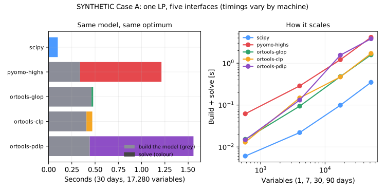
On 30 days (17,280 variables) the solvers take milliseconds; most of the time goes to building the model in Python (Pyomo, OR-Tools) or translating it for the solver. SciPy, which takes matrices directly, is fastest end to end. Pyomo buys readability and solver independence with build time. For a model re-solved every five minutes, that trade-off is real (Engineering track: latency budgets).
Two solvers, one process: a dependency trap
OR-Tools bundles its own copy of HiGHS (1.12.0); the highspy package that Pyomo uses
shipped a newer one. Loaded together in one Python process, whichever came second
crashed with an undefined symbol error. The fix here is to pin highspy to the same
version (highspy==1.12.0 in pyproject.toml). The general lesson for production: pin
solver versions, test the exact environment you deploy, and isolate incompatible
solvers in separate processes or containers.
The lesson
Write the model once, in the layer that suits the team, and keep the solver swappable. Then test across solvers: equal objectives, feasible solutions, cross-checked duals, stated gaps and tolerances. A solver is a component with versions, defaults and failure modes, not an oracle.
12 · Backtest
Nothing to backtest: this chapter is about how a model is solved, not whether its decisions were good. The solver-agreement tests are this chapter's regression suite.
13 · Adding realism
- Gurobi and CPLEX. The same Pyomo model runs on either by changing one string. Commercial solvers are faster on hard MIPs, not on this LP.
- Persistent solvers and warm starts. Re-solving every five minutes with small changes is faster if the model stays in the solver's memory (Pyomo's persistent interfaces, OR-Tools' incremental API).
- Other layers. PuLP and CVXPY (convex) for Python; JuMP in Julia; AMPL and GAMS commercially. The model-versus-solver split is the same.
- Problem structure. This LP separates into one tiny problem per interval. Exploiting structure (decomposition, T9) beats any solver on big models.
14 · Exercises
Guided
Build Chapter 1's single-interval problem (70 and 80 MW, $50 and $80/MWh, 100 MW) in Pyomo by hand and confirm $7,400/h and a $50/MWh shadow price.
Engineering
Add a backend: PuLP with its bundled CBC. Make it return a BackendResult and pass
the agreement tests.
Market
Give WF_A a participation coefficient of 0.8. Do all solvers still agree? What happens to the duals?
Challenge
Time 365 days on every backend. Where does each one spend its time, and which would you choose for a five-minute re-solve?
Production challenge
Write a CI job that runs the model on two different solvers and fails if the objectives differ by more than the stated tolerance, or a dual differs at a non-degenerate point.
15 · Production perspective
- Pin and record versions. Solver version, interface version and parameters belong in every run's log: they change answers at the tolerance level.
- Report status, gap and tolerance with every number.
SolveReportcarries them through the library. - Keep two solvers in CI. Disagreement is the cheapest bug detector you will ever have.
- Choose the layer for the team, the solver for the problem. Readability and testability usually beat a few milliseconds; integrality, size and licences decide the engine.
Run it yourself
| Artefact | Location |
|---|---|
| Case A in every backend | src/energy_or/toolbox/case_a.py |
| Synthetic days | src/energy_or/data/toolbox.py |
| Tests (solver agreement) | tests/test_toolbox.py |
| Notebook | notebooks/t1_one_model_many_solvers.ipynb |