7 · Lenders, covenants and the value of a dollar

Intermediate Parts XIII · XIV · XVII Cases H · L

In this chapter

• Follow a wind farm's cash through the waterfall: opex, lenders, then owners
• Turn the lender's DSCR covenants into the value of one more dollar, λ, with an exact formula
• See why λ can reach 1.5–2 for a farm close to lock-up and ≈ 1 for its neighbour
• Re-score Chapter 6's bidding policies by what reaches the owners rather than by revenue
• Decide how much room North should make for South, and see why the marginal value overshoots

Chapter 6 ended with a clear result. With no shortfall obligation, letting South run first behind the shared limit moves revenue from North to South and loses a little in total, so coordination is worth roughly nothing. That result counted every dollar the same, wherever it landed.

It doesn't hold when the two farms are financed separately. Each farm is its own project company with its own lenders, and a dollar earned by a farm about to fail its lender's test can be worth much more to its owner than a dollar earned by a farm with headroom.

Where this case comes from

The two farms are Chapter 6's, which follow an operating portfolio whose farms are financed separately. Budgets, debt terms, thresholds and costs here are synthetic, set at typical market levels; none comes from a real financing.

---

1 · The real-world problem

Banks lent against each farm's expected generation. Before lending, they had independent engineers estimate the long-run energy yield. The P50 is the level the farm should beat half the time; the P90 is a bad year it should beat nine years in ten. Debt is sized so that cash flow at P50 covers debt service comfortably, typically 1.30 times or more, and still covers it in a P90 year.

After financial close, the owner reports actual generation and revenue against a monthly budget. Twice a year the lenders test the debt service coverage ratio:

\[ DSCR = \frac{CFADS}{\text{debt service}} \]

where CFADS, cash flow available for debt service, is revenue minus operating costs.

DSCR at the test	What happens (typical)
≥ 1.30	On plan
< 1.15	Lock-up: no distributions to owners; cash is trapped in the project
< 1.05	Event of default: waivers, fees, margin step-ups, lender control

It is the end of March, halfway through the January–June test period. North is on budget. South had a poor quarter, at 85 % of budget revenue, and the constraint binds hard on windy days. Should North make room for South for the rest of the half, even though Chapter 6 showed that loses revenue?

2 · The system: a cash waterfall

flowchart TD
    R[Revenue: PPA + merchant] --> O[Operating costs]
    O --> C{{CFADS}}
    C --> D[Debt service: interest + principal]
    D --> T{DSCR test}
    T -- "≥ 1.15" --> E[Distribution to owners]
    T -- "< 1.15" --> L[Lock-up: cash trapped]
    T -- "< 1.05" --> X[Event of default]
    L -. "cured later, or swept to prepay debt" .-> E

Each farm has its own waterfall. Cash can't move from North's waterfall to South's: they are different companies, with different lenders, and possibly different co-owners. The only way to move value between them is through what each one earns in the market. That is the shared-limit bidding decision from Chapter 6.

3 · The decision

The same offers as Chapter 6, with one new number: θ, the share of the remaining constrained weeks in which North prices its displaced MW one cent behind South's offer, so that South runs first.

• θ = 0: each farm bids alone (Chapter 6's "local").
• θ = 1: South first in every constrained week.
• Anything in between: North makes room on some weeks, which in practice means stopping once South is safe.

4 · Variables and the four views

View	What it sees
Physical	MW behind a shared limit; nothing about the finance changes the network
Mathematical	CFADS as a random variable; a piecewise value function; θ ∈ [0, 1]
Optimiser	a one-dimensional search over θ, scored with exact expectations
Economic	lock-up and default probabilities for each farm, and who bears the risk

Symbol	Meaning	Units
\(C\)	CFADS for the test period	$
\(DS\)	debt service due in the period	$
\(L, D\)	lock-up and default DSCR	–
\(h\)	share of a trapped dollar's value lost to the owner	–
\(K\)	cost of a default to the owner	$
\(\lambda\)	value of one more dollar to the owner	–
\(\theta\)	share of constrained weeks in which North makes room	–

5 · The objective: what reaches the owners

The owner of a farm values the period's cash as

\[ V(C) = (C - DS)\,\big(1 - h\,\mathbb{1}[C < L\cdot DS]\big) \;-\; K\,\mathbb{1}[C < D\cdot DS] \]

The surplus after debt service is the owner's, unless the farm is locked up. Then the surplus is trapped, and a trapped dollar is worth \(1 - h\), because it arrives late if at all: repeated lock-ups often sweep trapped cash to prepay debt. A default costs a lump sum \(K\) more. We use \(h = 0.25\) and \(K = \$1\)M, both illustrative.

The objective is the sum of the two owners' expected values, not the sum of revenues.

6 · Constraints

• Physics, market and contracts: everything from Chapter 6 still holds. The shared limit, the price-ordered clearing, South's −$19.99 minimum offer and North's break-even.
• Market conduct: offers must follow the market's bidding and rebidding rules, including making offers in good faith. Making room changes where a farm offers, not what it reports about its plant.
• Each farm's finance documents: North's loan typically obliges it to operate prudently, and its lenders, and any co-owners, may object to it giving up revenue to help another company. The optimiser shows the trade-off; the decision belongs to both owners and, where the documents require it, their lenders.

7 · Formulation

Why these techniques? Structure → method

Property of the problem	Here	So
Decision	one number, the share \(\theta \in [0, 1]\) of constrained weeks in which North makes room	a one-dimensional search; no solver is needed
Objective	the owners' expected value \(V(C)\), which has jumps at the lock-up and default tests	not linear and not concave, so LP and convex duality do not apply to the whole problem
Uncertainty	the period's CFADS, treated as normal around the settled months	expectations of thresholds have a closed form (\(\Phi\), \(\varphi\)): exact, and differentiable
Coupling	a covenant tests the sum over the period, so a dollar in any week counts the same; the two farms are coupled only through the transfer \(\Delta_k\)	one number per farm summarises the covenant: the value of a dollar \(\lambda\)
Variables and constraints	1 variable; the covenants are in the objective as payoffs, not as hard constraints	slack, surplus and artificial variables do not arise
Information	decided once, at the end of March, on a budget-versus-actual report	a static policy; re-deciding as actuals arrive is left to the backtest
Speed	21 candidate values of \(\theta\), each evaluated in closed form	instantaneous, and easy to audit

Chosen. - The value of a dollar \(\lambda\) is the derivative of the owner's expected value with respect to a certain extra dollar. It plays the role a Lagrange multiplier plays in an LP: the price of relaxing the covenant, here the price of cash near a test. It tells the desk which way to move. - Closed-form expectation under a normal CFADS gives \(\lambda\) and \(\mathbb{E}[V]\) exactly, with no simulation noise in the derivative. - A grid search over \(\theta\) finds the best trade-off against the full value functions. In one dimension it needs no convexity: it simply compares candidates.

Not chosen. - Lagrangian relaxation or a MILP with a binary for "locked up". A covenant that must hold would be a constraint to relax. Here a breach is allowed and has a price, so it enters the objective, and a one-variable problem needs no integer machinery. - Chance-constrained programming. It would forbid breaches above a probability. Owners accept some risk at a price, and the question is what a dollar is worth, not whether risk is allowed. - Monte Carlo simulation of the whole waterfall. Correct but noisy: a derivative by finite differences on simulated payoffs near a jump is unreliable. Simulation remains the check for the normality assumption. - \(\lambda \times\) value per MWh as the final answer. The chapter shows it predicts +$105k where the real figure is +$27k, because \(\lambda\) is only a small-change price.

What the theory guarantees. - Under the normal assumption, \(\lambda\) is the exact derivative, so it gives the right direction. Because \(V\) is not concave, it does not give the right distance, which is why \(\theta\) is chosen against the full function. - A shared loan would give one waterfall and one \(\lambda\), and the problem would collapse to Chapter 6's ranking.

References. - Boyd and Vandenberghe (2004), Convex Optimization, chapter 5 and section 5.6: why a multiplier is a price, and when that reading holds (Chapter 7). - Choosing a technique for when a constraint becomes a payoff instead.

Halfway through the period, part of the CFADS is known and the rest depends on the wind. Treat the period's CFADS as normal, \(C \sim \mathcal{N}(\mu, \sigma^2)\), with the settled months fixed and each remaining month uncertain around budget (a 20 % coefficient of variation). Using \(\mathbb{E}[(C - a)\mathbb{1}(C < b)] = (\mu - a)\Phi(z) - \sigma\varphi(z)\) with \(z = (b - \mu)/\sigma\):

\[ \mathbb{E}[V] = (\mu - DS) - h\big[(\mu - DS)\Phi(z_L) - \sigma\varphi(z_L)\big] - K\,\Phi(z_D) \]

with \(z_L = (L\cdot DS - \mu)/\sigma\) and \(z_D = (D\cdot DS - \mu)/\sigma\). Differentiating with respect to a certain extra dollar gives the value of a dollar:

\[ \lambda = 1 - h\,\Phi(z_L) + h\,(L - 1)\,DS\,\frac{\varphi(z_L)}{\sigma} + K\,\frac{\varphi(z_D)}{\sigma} \]

Read it term by term:

• the first two terms are the share of a dollar that reaches the owner;
• the third is the value of lowering the probability of lock-up;
• the fourth is the value of lowering the probability of default.

Far from the thresholds λ = 1. Close to them, λ can be well above 1.

The decision is then a one-dimensional problem. With \(\Delta_k\) the revenue change farm \(k\) sees if North makes room in every remaining constrained week:

\[ \max_{\theta \in [0,1]} \;\; \sum_{k \in \{N, S\}} \mathbb{E}\big[V_k(C_k + \theta\,\Delta_k)\big] \]

\(\Delta_N < 0 < \Delta_S\), and \(\Delta_N + \Delta_S < 0\): making room always costs revenue. The library evaluates each candidate θ exactly, using the closed form above.

8 · Visualisation

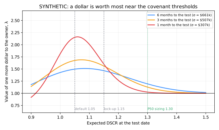
On plan, at DSCR 1.30, a dollar is worth about a dollar. As the expected DSCR falls towards the thresholds, λ climbs: a dollar now moves the probability of lock-up and default. It peaks near the default threshold, because \(K\) dominates, then falls again for a farm that is past saving, where a dollar is mostly trapped. The closer the test date, the less uncertainty is left, and the sharper and taller the peak.

9 · Implementation

from energy_or.data.contracts import NORTH, SHARED_LIMIT_MW, SOUTH, two_ppa_week
from energy_or.data.finance import CONSTRAINED_WEEKS_REMAINING, NORTH_FINANCE, SOUTH_FINANCE
from energy_or.finance import value_of_a_dollar
from energy_or.finance.coordination import evaluate_coordination, weekly_transfers

# South at 85 % of budget after three months (end of March)
outlook = SOUTH_FINANCE.outlook(months_elapsed=3, achievement_to_date=0.85)
lam = value_of_a_dollar(outlook, SOUTH_FINANCE.debt)  # ≈ 1.51

# Revenue each farm gains or loses per constrained week if North makes room
weeks = [two_ppa_week(seed=s) for s in (31, 32, 33)]
transfers = weekly_transfers([NORTH, SOUTH], weeks, SHARED_LIMIT_MW)

result = evaluate_coordination(
    [NORTH_FINANCE, SOUTH_FINANCE],
    transfers,
    months_elapsed=3,
    achievement_to_date=[1.0, 0.85],
    constrained_weeks=CONSTRAINED_WEEKS_REMAINING,
)
result["finance"].sacrifice_share  # θ* = 0.65

Artefact	Location
Covenants, owner value, λ	src/energy_or/finance/covenants.py
Policies scored through the covenants	src/energy_or/finance/coordination.py
Synthetic budgets and debt	src/energy_or/data/finance.py
Weighted ranking hook	value_weights in src/energy_or/contracts/bidding.py
Tests	tests/test_finance.py

10 · Solve

The budgets (synthetic, January–June):

	North	South
Budget revenue	$17.3M	$8.05M
Operating cost	$4.3M	$2.7M
CFADS at P50	$13.0M	$5.40M
Debt service (sized at 1.30)	$10.0M	$4.15M
CFADS that triggers lock-up	$11.5M	$4.77M

The outlook at the end of March. South's three months at 85 % of budget leave a $0.55M hole, and the remaining three months carry \(\sigma \approx \$0.51\)M:

South, revenue to date	Expected DSCR	P(lock-up)	P(default)	λ
100 %	1.30	11 %	2 %	1.13
95 %	1.26	19 %	5 %	1.23
90 %	1.21	31 %	9 %	1.36
85 %	1.17	44 %	17 %	1.51
80 %	1.12	59 %	27 %	1.63

North, on budget, has an 8 % chance of lock-up and λ ≈ 1.06.

The transfer. On Chapter 6's three constrained weeks, putting South first moves $103k a week to South for $121k a week of North's revenue. That is $1.18 of North per dollar for South, because North's contract pays more per MWh. Four constrained weeks like these are assumed left in the half.

The decision, North on budget and South at 85 %:

Policy	θ	Revenue change	North owner	South owner	Owners combined	P(lock-up) South	P(lock-up) North
Chapter 6, dollar ranking	–	≈ $0	−$1k	+$2k	≈ $0	44 % → 44 %	8 % → 8 %
South first, always	1	−$75k	−$526k	+$553k	+$27k	44 % → 17 %	8 % → 18 %
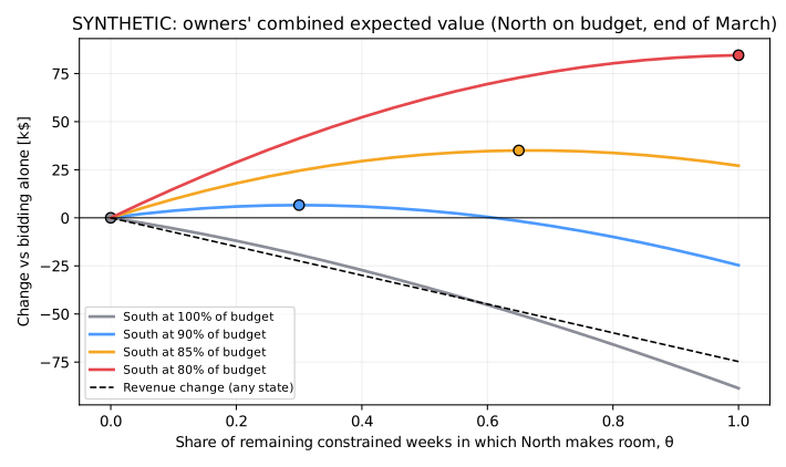
Finance-aware	0.65	−$49k	−$339k	+$374k	+$35k	44 % → 25 %	8 % → 14 %

11 · Interpret

The finance changes the answer, but only in distress

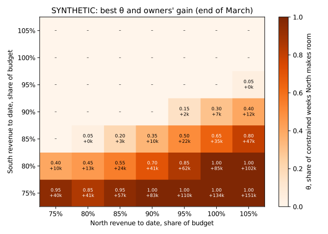
With South on budget, the best θ is 0, and South-first bidding destroys $89k of owner value. It gives up $75k of revenue and pushes North's lock-up risk up from 8 % to 18 % to shave a little off a South risk that was already small. With South at 85 %, making room on about two-thirds of the constrained weeks is worth +$35k to the owners while losing $49k of revenue. South's lock-up risk almost halves.

The map shows the whole picture. Coordination pays only in the lower right, where South is behind and North has headroom. When both farms are behind, North's own λ rises, and the case for helping South shrinks.

λ tells you the direction; curvature tells you how far

A tempting shortcut is to rank each MWh by λ × value per MWh: South's 1.51 against North's 1.06 easily beats the 1.18 exchange rate, so South first, always. Multiplying the full South-first transfer by those λs predicts +$105k. The real figure is +$27k, for three reasons:

• λ is a derivative, valid for a small change.
• The transfer is large, about 0.8σ of South's outlook, so South's λ falls as it is rescued.
• North's λ rises as it gives up revenue, and its lock-up risk doubles.

Optimising θ against the full value functions finds the point where the two marginal values meet, at θ = 0.65.

Shared loan, or one owner taking the whole view

If both farms sat under one loan, there would be one waterfall and one λ. A dollar would be worth the same in either farm, and the decision would collapse back to Chapter 6's dollar ranking, where coordination is worth ≈ 0. Separate financing is what creates the value, and it is also what makes the decision a governance question: North's owner and lenders bear the cost.

The lesson

Measure decisions by what reaches the owner, not by revenue. With separately financed assets, the value of a dollar depends on how close each project is to its covenants, so the right bidding strategy depends on the budget-vs-actual report as much as on the price forecast. And use the marginal value to see which way to move, then optimise against the full value function to see how far.

Next: turning it into a bid

θ and the λs say what to do. Chapter 8 turns it into MW per price band, with band prices fixed the day before.

12 · Backtest

Nothing here has been backtested. A real test would need:

• each farm's actual monthly revenue against budget;
• the covenant definitions from the finance documents (most test a trailing twelve months, not one half);
• archived predispatch, to replay the offers the desk would have made each week, with θ re-chosen as actuals arrived.

That needs the common backtesting framework (Milestone 7) and the rolling-horizon machinery (Milestone 9). The policy here is static: θ is chosen once, at the end of March.

13 · Adding realism

1. Trailing-twelve-month DSCR and multiple tests. A dollar earned now counts in two tests, so λ sums over both.
2. Debt service reserve accounts. A funded DSRA softens a default but has to be refilled from future cash.
3. Cash sweeps. Repeated lock-ups sweep trapped cash to prepay debt, so \(h\) grows with each failed test.
4. P90 sizing and sculpting. Debt service varies by period with the budget, so the test period matters.
5. Correlated wind. North and South share weather, so their shortfalls coincide. That is exactly when helping South is hardest, as the map's lower-left corner shows.
6. Ownership splits and tax. If the co-owners differ, the "owners combined" objective needs weights, or a side agreement between them.

14 · Exercises

Guided

South at 85 %, three months left: compute \(z_L\), \(z_D\) and λ by hand from the table in §10, and check against value_of_a_dollar.

Engineering

Replace the normal CFADS with a Monte Carlo over monthly revenue (lognormal, 20 % CV), and check that the closed-form \(\mathbb{E}[V]\) and λ agree within sampling error. When would the normal assumption mislead?

Market

Set \(K = 0\) (a default costs nothing beyond lock-up) and then \(K = \$3\)M. How do θ* and the map change? Which assumption is the decision most sensitive to?

Challenge

Make θ adaptive. Re-choose it every week from the updated outlook, simulated over many weather paths. How much better is the adaptive policy than the static one, and when does it stop making room?

Production challenge

The desk sets θ weekly from the finance team's budget-vs-actual report. Design the data contract between the two systems, the approval step (who signs off on North giving up revenue), and what each decision logs so lenders and auditors can see why it was taken.

15 · Production perspective

• Finance as an input to dispatch. Publish each project's λ weekly, from the same budget-vs-actual system the finance team reports from. A stale λ is as dangerous as a stale price.
• Measure decision value. Report revenue and owner value per project, with lock-up and default probabilities before and after, so a revenue loss that buys a covenant pass is visible as such.
• Governance first. Any policy that lowers one project's revenue for another's benefit needs a documented approval from both owners, and from the lenders where required. The system's job is to make the trade-off explicit, not to decide it.
• Respect the envelope. Market rules, the contracts and each project's finance documents bound every decision; the optimiser only chooses among permitted offers.

Run it yourself

Artefact	Location
Covenant model	src/energy_or/finance/covenants.py
Coordination scoring	src/energy_or/finance/coordination.py
Synthetic budgets	src/energy_or/data/finance.py
Tests	tests/test_finance.py
Notebook	notebooks/07_lenders_and_covenants.ipynb