1 · Two wind farms, one connection

Foundation Case A Linear programming

In this chapter

• Turn an operational question into decision variables, an objective and constraints
• See a linear program as a shape (the feasible region) and a direction (the objective)
• Understand why the optimum sits on a corner and which constraints are binding
• Meet the shadow price: what one more MW of network is worth, and why it equals the value of the marginal farm
• Compare the optimiser with a common real-world rule (pro-rata curtailment) over a synthetic day

---

1 · The real-world problem

Two wind farms, WF_A and WF_B, sit next to each other and export through a shared piece of network: a connection asset rated at 100 MW. Right now the wind is up. WF_A could produce 70 MW and WF_B could produce 80 MW: 150 MW of available energy trying to squeeze through 100 MW of network.

Something has to give. 50 MW will be curtailed. The question is whose.

If both farms were identical, the answer would not matter much. They are not. Each megawatt-hour WF_B exports is worth $80 to its owner, and each one WF_A exports is worth $50. Why would identical megawatt-hours be worth different amounts? Because the farms have different commercial positions:

	WF_A	WF_B
Commercial position	Merchant: sells at spot, plus LGCs	Pay-as-produced PPA, LGCs bundled
Illustrative build-up	$40 × MLF 0.95 + $12 LGC ≈ $50/MWh	$80/MWh PPA price
Value to owner, \(v\)	$50/MWh	$80/MWh

Illustrative numbers

These values are simplified on purpose. How spot, MLFs, LGCs and PPAs really combine (and why a PPA can make a generator's rational behaviour differ from a merchant one) is the subject of Parts XIV and XV. For now, treat each \(v\) as a given number.

2 · The physical system

Both farms connect to the same connection asset, say a shared substation transformer. Thermal rating limits the total power through it. Each farm's power plant controller can be given an active-power setpoint, so the operator can choose how much each farm exports, up to whatever the wind allows.

Two kinds of limit apply:

• Availability: a farm cannot export more than its turbines can make from the current wind (in NEM terms, roughly what a UIGF-style availability forecast predicts).
• Shared limit: the sum of the two exports cannot exceed the connection's rating.

Who decides in the real NEM?

In this chapter the owner controls the allocation because the limit is a private connection asset. When the limiting element is part of the shared transmission network, AEMO's dispatch engine (NEMDE) decides, using participants' offers and published constraint equations. NEMDE also solves a linear program, which is why this chapter is the right foundation, but nothing here reproduces NEMDE. Network constraints in the market get their own part of the book (Part XIII).

3 · The decision

For this dispatch interval, what active-power setpoint should each farm receive?

That is all. The weather, the prices and the connection rating are given. The only thing we control is how the 100 MW is shared.

4 · Decision variables

Symbol	Meaning	Units
\(P_A\)	Export from WF_A this interval	MW
\(P_B\)	Export from WF_B this interval	MW

A decision variable is a quantity the optimiser is allowed to choose. Everything else is a parameter: data we take as fixed.

Parameter	Meaning	Value
\(L\)	Shared connection limit	100 MW
\(\bar P_A,\ \bar P_B\)	Available capacity	70 MW, 80 MW
\(v_A,\ v_B\)	Value per MWh exported	$50/MWh, $80/MWh

5 · Objective

We want as much value as possible. If the farms export \(P_A\) and \(P_B\) MW for one hour, the value earned is

\[ 50 P_A + 80 P_B \quad [\$/\text{h}]. \]

Units first, always

\(v\) is in $/MWh and \(P\) is in MW, so \(vP\) is in $/h, a rate. A NEM dispatch interval lasts five minutes, so the value actually earned in one interval is \(vP \times \tfrac{5}{60}\). Getting the 12× wrong produces plausible-looking numbers that are simply wrong. The library keeps the two quantities apart: value_rate_per_h and value_per_interval(minutes=5).

6 · Constraints

A constraint is simply something the optimiser is not allowed to violate.

Constraint	Physical meaning
\(P_A + P_B \le 100\)	The connection cannot carry more than 100 MW
\(P_A \le 70\)	WF_A cannot export more than the wind gives it
\(P_B \le 80\)	WF_B cannot export more than the wind gives it
\(P_A,\ P_B \ge 0\)	Wind farms export, they do not import

7 · Mathematical formulation

Why these techniques? Structure → method

Property of the problem	Here	So
Objective	\(50P_A + 80P_B\): a constant times each variable	linear, so a linear programme (LP) and not a nonlinear one
Variables	two, both continuous (MW)	2 variables: the graphical method works. With 288 (a day of 5-minute intervals) or 2 million it cannot be drawn, so a solver needs an algebraic method
Constraints	three of the form \(\le\), plus \(P \ge 0\)	each \(\le\) row gets a slack variable, \(P_A + P_B + s_1 = 100\); the origin is then a feasible starting corner
Other constraint types	none here	a \(\ge\) row needs a surplus variable, and \(\ge\) or \(=\) rows need an artificial variable (big-M or two-phase) to find a first corner
Feasible region	a bounded polygon with 5 corners	the optimum is at a corner (fundamental theorem), so searching corners is enough
Time coupling and uncertainty	none: one interval, known availability	no stages, no scenarios
Size and speed	2 variables, 3 rows, about 3 ms	any LP solver is instant; the method matters for the later chapters, not for speed here

Chosen. - The graphical method solves this model by eye: draw the three half-planes, slide the objective line, and read off the corner (20, 80). It is chosen because it shows why the optimum is a corner and what a binding constraint is. - The simplex method is what a solver does instead of drawing. It adds one slack variable per \(\le\) row, starts at the origin and moves along edges to a neighbouring corner that improves the objective, stopping when none does. T0 · The simplex method by hand works this model through step by step and generalises the corner-walking to any number of variables, including \(\ge\) and \(=\) rows. - LP duality gives the shadow prices, read from the same solve at no extra cost.

Not chosen. - Interior-point methods. They cross the inside of the region and are fastest on very large LPs. For three rows they add nothing, and they return a point that is not a corner, which hides the binding set this chapter wants to show. - Nonlinear or gradient methods. Nothing in the problem is curved. A gradient method would stall on the flat objective edges and give no certificate of optimality. - A rule such as pro-rata curtailment. It is simple and transparent, but it ignores the values \(v\) and so cannot be optimal. Section 12 measures the loss. - Enumerating corners. With \(n\) variables and \(m\) rows there can be on the order of \(\binom{n+m}{m}\) of them. Simplex visits only an improving few.

What the theory guarantees. If an LP has an optimum and a corner, some corner is optimal (Dantzig, 1963; Bertsimas and Tsitsiklis, 1997). The simplex method finds it in finitely many steps once a rule such as Bland's prevents cycling at degenerate corners. Its worst case is exponential (Klee and Minty, 1972), but practice is far better, and interior-point methods are polynomial (Karmarkar, 1984). Strong duality means the dual value equals the primal value at the optimum, so the shadow prices come with a proof.

References. - Bertsimas and Tsitsiklis (1997), Introduction to Linear Optimization: the geometry of corners, the simplex method and duality (Chapter 1). - Dantzig (1963), Linear Programming and Extensions: simplex, slack variables and the tableau (Choosing a technique). - Bland (1977), anti-cycling pivot rules; Klee and Minty (1972), worst-case behaviour; Karmarkar (1984), interior points (same section). - Kirschen and Strbac (2019), Fundamentals of Power System Economics: why a shadow price of a network limit is a marginal value (Chapter 1). - Choosing a technique for how structure decides the method across the whole book.

Putting it together gives a linear program (LP):

\[ \begin{aligned} \max_{P_A,\,P_B}\quad & 50P_A + 80P_B \\ \text{s.t.}\quad & P_A + P_B \le 100 && \text{(shared limit)} \\ & P_A \le 70 && \text{(WF_A availability)} \\ & P_B \le 80 && \text{(WF_B availability)} \\ & P_A,\ P_B \ge 0. \end{aligned} \]

It is linear because every term is a constant times a variable: no \(P^2\), no \(P_A P_B\), no on/off switches. Linearity is what makes LPs fast and reliable to solve, even with millions of variables.

The same problem in matrix form, \(\max\, c^\top x\) subject to \(Ax \le b,\ x \ge 0\):

\[ c = \begin{bmatrix}50\\80\end{bmatrix},\qquad A = \begin{bmatrix}1&1\\1&0\\0&1\end{bmatrix},\qquad b = \begin{bmatrix}100\\70\\80\end{bmatrix}. \]

Each row of \(A\) is one constraint. Each column is one decision variable. This is the form every LP solver works with, and it scales unchanged from 2 variables to 2 million.

General form, for any number of farms

With farms \(i = 1,\dots,n\), participation coefficients \(a_i\) (how strongly each farm loads the limiting element; all 1 here):

\[ \max_{P}\ \sum_i v_i P_i \quad\text{s.t.}\quad \sum_i a_i P_i \le L,\quad 0 \le P_i \le \bar P_i. \]

energy_or.network.solve_shared_connection implements exactly this.

8 · Visualisation

With two variables, every possible decision is a point on a plane: \(P_A\) across, \(P_B\) up. Each constraint cuts the plane in half. What survives all the cuts is the feasible region: every decision that breaks no rule.

The objective \(50P_A + 80P_B = k\) is a family of parallel lines, one for each value \(k\). Increasing \(k\) slides the line up and to the right. The best decision is the last point of the feasible region the line touches before leaving it.

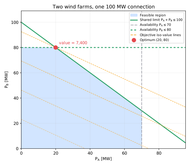
The last point touched is the corner (20, 80). That is not a coincidence:

The fundamental theorem of linear programming

If an LP has an optimal solution and its feasible region has a corner, then some corner is optimal. Solvers exploit this: the simplex method walks from corner to corner, improving the objective at each step.

Explore it yourself

Move the sliders. Watch the region change shape, the optimum jump between corners, and the binding constraints (green) change.

Things to try:

• Raise WF_A's value above WF_B's. The optimum jumps to the other corner.
• Set the two values equal. The objective line becomes parallel to the shared-limit edge, and every point on that edge is optimal.
• Push the limit above 150 MW. The shared limit stops binding and its marginal value drops to zero.
• Make WF_A's value negative (think negative spot price with no LGC). WF_A is curtailed even though there is spare network.

9 · Python implementation

The model lives in the library, not in the notebook, so the book, the notebook, the figures, the animation and the tests all use the same code.

from energy_or.network import Generator, solve_shared_connection

farms = [
    Generator("WF_A", available_mw=70, value_per_mwh=50),
    Generator("WF_B", available_mw=80, value_per_mwh=80),
]
result = solve_shared_connection(farms, limit_mw=100)

Under the hood (src/energy_or/network/shared_connection.py) this builds a named LinearProgram: one variable per farm, one shared_limit row and one avail_<farm> row per farm. Then it calls the open-source HiGHS solver through scipy.optimize.linprog. Naming every constraint matters: it is what lets us say which constraint is binding instead of "row 0".

10 · Solve

print(result.explain())

RECOMMENDATION

  WF_A     export   20.00 MW of   70.00 MW available  (curtail  50.00 MW, value $50.00/MWh)
  WF_B     export   80.00 MW of   80.00 MW available  (curtail   0.00 MW, value $80.00/MWh)

  Value rate:        $7,400.00/h  ($616.67 per 5-minute interval)

Binding constraints:
  • shared_limit
  • avail_WF_B

Marginal values (shadow prices):
  • +1 MW of shared capacity  → +$50.00/h
  • +1 MW available at WF_A   → +$0.00/h
  • +1 MW available at WF_B   → +$30.00/h

Solver: HiGHS (scipy.optimize.linprog), status optimal, 2 variables, 3 constraints, 2.7 ms

11 · Interpret

What did the optimiser choose, and why?

WF_B runs flat out at 80 MW. WF_A gets the remaining 20 MW and is curtailed by 50 MW. The logic is a merit order: give the scarce network to whoever values it most, until they cannot use any more, then move to the next.

Which constraints were binding?

A constraint is binding when the optimum sits exactly on it: it is "full".

• Shared limit: binding. All 100 MW are used.
• WF_B availability: binding. B is exporting everything the wind gives it.
• WF_A availability: not binding. A has 50 MW of slack.

Non-binding constraints do not affect the answer locally. You could loosen \(P_A \le 70\) to \(P_A \le 1000\) and nothing would change.

Shadow prices: what is one more MW worth?

The shadow price (or dual value, or marginal value) of a constraint is how much the optimal objective improves if that constraint is relaxed by one unit.

Constraint	Shadow price	Why
Shared limit	$50/MWh	One more MW of network goes to WF_A, the marginal farm, worth $50
WF_B availability	$30/MWh	One more MW at B displaces one MW of A: \(80 - 50\)
WF_A availability	$0/MWh	A already has spare availability; more is useless

The first row is the most important idea in this chapter:

The value of network capacity is set by the marginal generator

WF_B's MWh are worth $80, but extra network is worth only $50, because WF_B is already full. The marginal unit, the one partly dispatched and partly curtailed, sets the price of the constraint. The same logic, applied to a whole region and to offers instead of private values, is how marginal prices form in electricity markets.

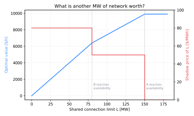
Shadow prices are only valid locally. Plot the optimal value against the limit \(L\) and the slope (the shadow price) changes in steps:

Limit \(L\)	Who is marginal	Shadow price of \(L\)
0 – 80 MW	WF_B (A is fully curtailed)	$80/MWh
80 – 150 MW	WF_A	$50/MWh
> 150 MW	nobody: the limit no longer binds	$0/MWh

The value curve is concave and piecewise linear. Every extra MW is worth no more than the last one. That shape is general to LPs, and it is why the first few MW of network augmentation are always the most valuable.

Advanced: degenerate corners

At exactly \(L = 80\) or \(L = 150\), three constraints meet at the optimum and the shadow price is not unique: the left and right slopes differ. A solver will report one valid value, which may not be the one you expect. Production code that consumes duals must handle this (Part II, sensitivity analysis).

Translate back to operations

For one 5-minute interval at these conditions:

• Curtailed energy: \(50\text{ MW} \times \tfrac{5}{60}\text{ h} = 4.17\text{ MWh}\), all at WF_A.
• Value earned: $616.67.
• Curtailment here is an opportunity loss, not a fault. WF_A was available but the network was not. Keep technical availability, commercial availability, dispatch target and actual generation apart; they are different things.

12 · Backtest: LP versus pro-rata

A real comparison against plant history needs SCADA and contract data, which this book cannot publish. Instead we compare the LP with a very common operating rule, pro-rata curtailment (every farm is cut by the same fraction of its availability), on one day of synthetic 5-minute data.

Synthetic / illustrative data

The availability and price series come from energy_or.data.synthetic.two_farm_day(seed=7). They are shaped to look plausible and must not be read as real plant or market history.

In this day, WF_A's value follows spot (\(0.92 \times RRP + \$15\)) and WF_B is on a flat $65/MWh PPA. So the merit order flips during the day: overnight and in the evening peak WF_A is worth more; in the midday solar trough WF_B is.

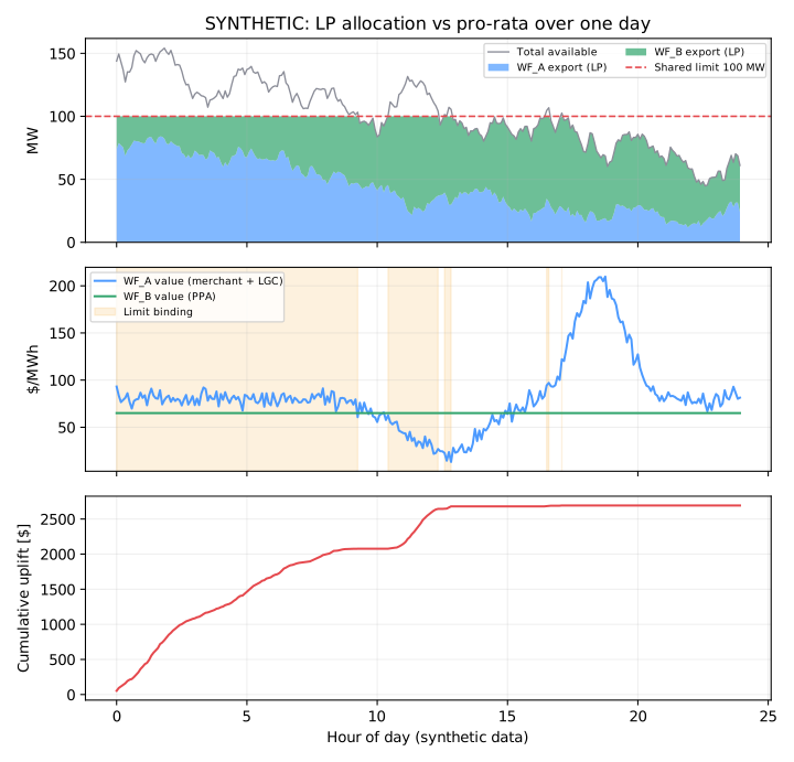
Over this synthetic day the limit binds in about half of all intervals. The LP earns about $2,700 (≈ 1.8 %) more than pro-rata. In intervals where the limit does not bind, the two policies are identical; all of the uplift comes from who gets curtailed when someone must be. And the LP is never worse in any interval. That is not luck; it is what optimal means, and the test suite checks it on every commit.

What this backtest does not show

Each interval is solved with perfect knowledge of that interval's availability and value. A real controller sets targets using forecasts. A proper backtest must only use information available at decision time. Building that discipline is Part XIX.

13 · Adding realism

Each of these is a small change to the model. Several are already supported by the library.

1. Participation coefficients. Real constraint equations weight each unit by how much it loads the limiting element: \(a_A P_A + a_B P_B \le L\). With \(a_A = 0.5\), WF_A earns \(50 / 0.5 = \$100\) per MW of limit used, more than WF_B's $80. A now gets priority, even though its MWh are worth less. Merit order is value per unit of the scarce resource, not value per MWh. (Try it: Generator(..., coefficient=0.5).)
2. Negative values. At negative spot prices a merchant farm without LGCs loses money on every MWh. The LP curtails it voluntarily; the shared limit stops binding.
3. Marginal loss factors. Scale spot revenue by each farm's MLF. Two farms seeing the same regional price can value an MWh differently.
4. Time coupling. Here every interval is independent. Add ramp-rate limits, or a battery behind the same connection, and decisions in one interval constrain the next. That is where Chapter 2 (BESS) begins.
5. Uncertainty. Availability is a forecast. If WF_B's forecast is 80 MW but it actually delivers 70 MW, 10 MW of network sits idle. Part IV forecasts it; Part XVII optimises against the uncertainty.

14 · Exercises

Guided

Before running anything, predict the optimal dispatch and the shadow price of the shared limit when \(L = 60\) MW. Then check with the explorer or the notebook.

Engineering

WF_A has a minimum stable export of 10 MW whenever it is online. Why can this not be written as a single linear constraint? (Hint: "either 0 or at least 10".) This is the doorway to mixed-integer programming.

Market

The spot price falls to −$30/MWh. WF_A is merchant with LGCs worth $35/MWh; WF_B's PPA pays $65/MWh regardless. Compute \(v_A\) and the optimal dispatch. Does the shared limit bind?

Challenge

Add a third farm, WF_C (available 40 MW, value $60/MWh, coefficient 0.8). Solve it with solve_shared_connection, then explain the merit order using value per MW of limit.

Production challenge

This LP solves in about 3 ms. Suppose it must run every 5 minutes for 40 farms behind 15 overlapping limits, using availability forecasts that arrive 20 seconds before the interval starts. List what could go wrong (late data, infeasibility, stale forecasts) and what the system should do in each case.

15 · Production perspective

A model that solves once in a notebook is not yet a decision system. To run this continuously you would need to:

• Ingest availability forecasts and prices every interval, and validate them: missing intervals, negative availability, a forecast far above nameplate.
• Solve within a latency budget, and record the SolveReport: status, solve time, problem size. A non-optimal status must trigger a safe fallback, such as pro-rata, never silence.
• Act within the permitted envelope: setpoints must respect plant and connection agreement limits, whatever the optimiser says.
• Explain: log binding constraints and shadow prices, so a control-room operator can see why WF_A was curtailed.
• Measure: compare actual exports with targets, and backtest the policy against history.

Engineering Lab 1 takes the first step: turning this model into a tested, typed package with CI.

Run it yourself

The notebook notebooks/01_shared_connection_lp.ipynb solves the reference problem, draws the feasible region, sweeps the limit to trace the value curve, and runs the synthetic-day comparison. Change anything.

Artefact	Location
Model	src/energy_or/network/shared_connection.py
Generic LP layer	src/energy_or/optimisation/lp.py
Tests (hand-derived optima)	tests/test_shared_connection.py
Animation	animations/foundations/feasible_region.py
Figures	scripts/build_figures.py