3 · Reliability, availability and when to replace
Foundation Intermediate Part VII–VIII Cases C · D

In this chapter
- Availability from MTBF and MTTR, and why time-based and energy-based availability differ
- Failure rates with honest uncertainty: a handful of failures says very little
- The Weibull distribution and the hazard function: infant mortality, random failure, wear-out
- Censoring: the turbines that have not failed yet are data too
- Maintainability: right-skewed repair times, and what a faster response is worth
- The first economic reliability decision: when should a gearbox be replaced before it fails?
This chapter is less about solvers and more about the inputs every maintenance, logistics and fleet model later in the book depends on. A maintenance optimiser fed with a failure rate of "0.4 per year" behaves very differently from one fed with "somewhere between 0.08 and 1.3 per year". Getting the reliability model right comes before optimising anything.
1 · The real-world problem
A 28-turbine wind farm stops, on average, about a hundred times per turbine per year for five minutes or more. Most stops are grid or park-controller commands and self-clearing alarms lasting minutes. A few are multi-week outages waiting for a part, a specialist or a crane, and they cause most of the lost energy. The O&M contract guarantees an energy-based availability in the high 90s. The site manager's questions are:
- Which stops actually cost us energy, and money? If we could go back in time, what would we fix first?
- Would a faster technician response pay for itself, or spares held on site?
- Our gearboxes are ageing. Should we replace them before they fail?
The third question is the one an optimiser answers. But the first two decide whether its inputs are right.
Where the numbers come from
The synthetic farm in this chapter is calibrated to anonymised aggregates from the SCADA event logs and downtime reports of operating ~28-turbine Australian wind farms: stop rates by turbine system, duration percentiles, the long tail of outages waiting for parts, repeat faults, how concentrated losses are on a few turbines, and achieved availability. No real event, turbine, site or contract value appears in the book. The calibration is shown in Section 5.
2 · The physical system
A turbine alternates between two states:
stateDiagram-v2
    direction LR
    Running --> Stopped: failure / alarm / planned work
Stopped --> Running: reset / repair / restart- Time to failure (TTF): how long it runs before stopping. Its mean is the MTBF, mean time between failures.
- Time to repair (TTR): how long it stays stopped. Its mean is the MTTR, and it includes waiting (for a technician, parts, a crane, a weather window) as well as hands-on work.
Reliability engineering models the first; maintainability engineering models the second. They are different disciplines with different levers: better components versus better logistics.
3 · The decision
Two decisions in this chapter:
- Maintainability. How fast should we respond to stops that need a technician? (A roster decision.)
- Replacement. At what operating age, if any, should a wearing component be replaced preventively? (A policy decision, and the first economic reliability optimisation in the book.)
4 · Availability: the first model
For a repairable item in steady state:
On the synthetic farm, a turbine stops every 81 hours on average and stays stopped 3.8 hours on average:
That number hides almost everything that matters:
A stop at 3 m/s is not a stop at 14 m/s. Time-based availability counts hours; energy-based availability counts the MWh that could have been produced. Planned work is deliberately scheduled in calm weather, so it costs little energy. But planned work is a small share of the downtime here: the multi-week outages run through windy and calm weeks alike, so the two measures end up close:
| Measure | Synthetic farm |
|---|---|
| Time-based availability | 95.70 % |
| Energy-based availability | 95.70 % |
Contracts increasingly guarantee energy-based availability, and add rules about which downtime counts: grid outages, owner-caused stops, out-of-spec weather and capped planned-maintenance allowances are typically excluded or deemed available. Contract definitions decide what "availability" means before any statistics do.
Keep the availabilities apart
Technical availability, contractual availability, commercial availability and actual generation are different quantities (see Notation and units). A model that mixes them produces confident numbers about the wrong thing.
5 · Where the lost energy goes
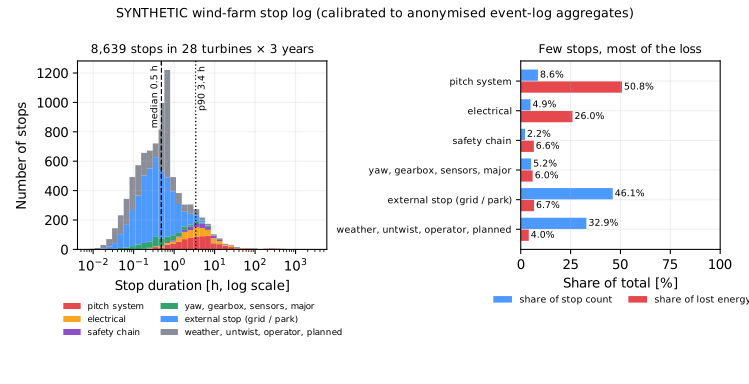
Stop durations are extremely right-skewed: the median stop lasts half an hour, the mean nearly four hours. Over three synthetic years, by turbine system:
| System | Stops / turbine-yr | Median | Share of stops | Share of lost energy |
|---|---|---|---|---|
| Pitch system (converters, batteries, pitch comms) | 8.9 | 3.8 h | 8.6 % | 50.8 % |
| Electrical (fuses, top box, converter) | 5.1 | 3.5 h | 4.9 % | 26.0 % |
| Safety chain / e-stop | 2.2 | 4.1 h | 2.2 % | 6.6 % |
| Yaw | 2.6 | 0.4 h | 2.5 % | 2.7 % |
| Major component (crane exchange) | 0.01 | 916 h | < 0.1 % | 2.2 % |
| Gearbox, sensors and other | 2.8 | 0.4 h | 2.7 % | 1.1 % |
| External stop (grid / park controller) | 47.4 | 0.3 h | 46.1 % | 6.7 % |
| Weather, cable untwist, operator, planned | 33.9 | 0.1–2.3 h | 32.9 % | 4.0 % |
Three patterns matter more than the averages:
- The loss is in the tail. Stops longer than 24 hours are 1 % of events but 69 % of lost energy. Stops shorter than an hour are three-quarters of events and 7 % of the energy. Reliability effort spent on the noisy alarm list, the most visible problem, is aimed at the smallest part of the loss.
- Most of the tail is waiting, not repairing. Half of all lost energy (53 %) is lost after the first 72 hours of an outage: waiting for parts, a specialist or a crane.
- A few turbines carry each problem. Three turbines cause half of the pitch system's lost energy, and a quarter of pitch stops come back within a day of the turbine restarting.
Calibration
The reference is the anonymised aggregate of a 28-turbine farm's SCADA event logs over 27 months (63 turbine-years). The model column is the mean of 20 synthetic three-year farms, with the 10th–90th percentile range in brackets.
| Statistic | Observed aggregate | Synthetic model |
|---|---|---|
| Stops ≥ 5 min per turbine-year | ≈ 98 | 91 (87–94) |
| Median stop (≥ 5 min) | ≈ 0.5 h | 0.55 h |
| 90th / 99th percentile | ≈ 3.8 h / 33 h | 3.5 h / 31 h |
| Outages > 24 h per turbine-year | ≈ 1.9 | 1.1 (0.9–1.4) |
| Outages > 48 h per turbine-year | ≈ 0.7 | 0.6 (0.5–0.8) |
| Outages > 100 h per turbine-year | ≈ 0.3 | 0.4 (0.3–0.6) |
| Time-based availability | ≈ 95.5 % | 95.9 % (95.0–97.0) |
| Energy lost | ≈ 4.6 % | 4.2 % (3.1–5.3) |
| Pitch system's share of lost energy | ≈ 46 % | 49 % (32–62) |
| Electrical share | ≈ 22 % | 28 % (15–38) |
| Lost after the first 72 h of an outage | ≈ 50 % | 52 % (43–62) |
| Pitch stops repeating within 24 h | ≈ 22 % | 22 % (17–26) |
| Top-3 turbines' share of pitch loss | ≈ 58 % | 62 % (50–71) |
| Weibull shape, time between pitch stops | ≈ 0.40 | 0.45 (0.42–0.50) |
The model reproduces the shape of the real data. Where it misses, it says something: real outages of one to four days are more common than the model makes them, because real repairs bunch at "next working day" and "after the weekend", which a lognormal can't produce. And the seed-to-seed ranges are wide, which is itself a lesson: the rare long outages that cause half the loss are exactly the part of the distribution any dataset estimates worst.
Why these techniques? Structure → method
This chapter is mostly statistics, with one small optimisation at the end. The table therefore asks what kind of question each part poses, not only whether it is an LP.
| Property of the problem | Here | So |
|---|---|---|
| Failures are counts over exposure | 2 outages in 56 turbine-months | a Poisson model with an exact interval (Garwood, 1936), because a normal approximation fails at small counts |
| Failure rate may change with age | gearboxes and bearings wear out | Weibull: one shape parameter \(\beta\) covers falling, constant and rising hazard |
| Some units have not failed | survivors are right-censored | censored maximum likelihood: survivors enter through \(\ln R(t_j)\) |
| Repair times | right-skewed, mean far above median | lognormal, fitted to log durations |
| Decision variable | one: the replacement age \(T\) | 1 variable: a curve can be drawn and searched; no LP, no slack or artificial variables because there are no constraints beyond \(T > 0\) |
| Objective | \(g(T)\), smooth and nonlinear (renewal-reward) | a grid, then a bounded scalar search |
| Uncertainty | the parameters \(\beta, \eta\) are themselves estimated | report intervals; optimise against a distribution later (Part XVII) |
| Size and speed | a few hundred failures; milliseconds | nothing here needs a heavy method |
Chosen.
- Poisson counts with chi-square limits. Failures per unit of exposure is the
natural statistic, and the interval is exact, so it stays valid for two failures as
well as for twenty.
- Weibull with censoring. The hazard \(h(t)\) is what a replacement decision uses,
and the Weibull makes it a one-parameter question: is \(\beta\) above 1? Censoring is
handled in the likelihood rather than by discarding survivors. Weibull.fit
maximises it with the derivative-free Nelder–Mead search on \((\ln\beta, \ln\eta)\).
- Age replacement via the renewal-reward theorem. It turns a stochastic life into
one number, a long-run cost per hour, which depends on a single decision \(T\).
- A grid plus a bounded scalar search, because the curve is smooth and
one-dimensional; the grid guards against a local minimum.
Not chosen. - A constant-rate (exponential) model for everything. It is right when \(\beta = 1\) and wrong for wear-out. Assuming it makes preventive replacement look pointless. - Fitting only the failed units. This discards the long lives and biases \(\eta\) low (the chapter's test shows \(\eta\) below 14 years against a true 20). - Kaplan–Meier alone. It is an excellent non-parametric survival curve, but it stops at the last observation. A replacement age needs the tail beyond it, which a parametric form extrapolates, with the risk that implies. - An LP or MILP for the replacement age. There is one variable and a nonlinear objective. Scheduling many replacements against a crane and spares is a MILP, and it starts in Chapter 5.
What the theory guarantees. The Poisson interval has coverage of at least the stated level (Garwood, 1936). The age-replacement problem has a finite optimum when the hazard is increasing and a failure costs more than a planned replacement; otherwise run-to-failure is best (Barlow and Hunter, 1960). Maximum likelihood is consistent with censored data, but with few failures it is imprecise, which the intervals show.
References. - Rausand, Barros and Høyland (2021), System Reliability Theory: availability, failure rates and maintenance models (Chapter 3). - Meeker and Escobar (1998), Statistical Methods for Reliability Data: censored likelihoods and Weibull and lognormal fits (same section). - Garwood (1936), exact Poisson limits; Weibull (1951), the distribution; Kaplan and Meier (1958), using survivors (same section). - Barlow and Hunter (1960), optimum preventive maintenance: the age-replacement result (same section). - Choosing a technique for how structure decides the method across the book.
6 · Failure rates, with honest uncertainty
The simplest reliability model has a constant failure rate \(\lambda\):
Exposure is turbine-time, not calendar time: 28 turbines for two months is 56 turbine-months. Suppose two outages longer than 100 hours occurred in that window:
from energy_or.reliability import failure_rate, HOURS_PER_YEAR

failure_rate(2, 56 * HOURS_PER_YEAR / 12).per_year
# (0.43, 0.08, 1.35)   estimate, 90 % lower, 90 % upper  [per turbine-year]
The point estimate is 0.43 per turbine-year, but the 90 % interval runs from 0.08 to 1.35, a factor of 18. With 20 failures over ten times the exposure, the same estimate has an interval of 0.28–0.62. The interval comes from the exact relationship between a Poisson count and the chi-square distribution:
Rule of thumb
Always report a failure rate with its interval and its exposure. Decisions that flip inside the interval need more data, or a decision that is robust to it (Part XVII).
7 · The Weibull distribution and the hazard function
A constant rate assumes age doesn't matter. For gearboxes, bearings and blades, it does. The Weibull distribution has two parameters:
- Shape \(\beta\): how the failure rate changes with age.
- Scale \(\eta\): the characteristic life. 63.2 % have failed by \(t = \eta\).
\(R(t)\) is the reliability: the probability of surviving past age \(t\). \(h(t)\) is the hazard: the failure rate among survivors at age \(t\). The hazard is the quantity maintenance decisions depend on.
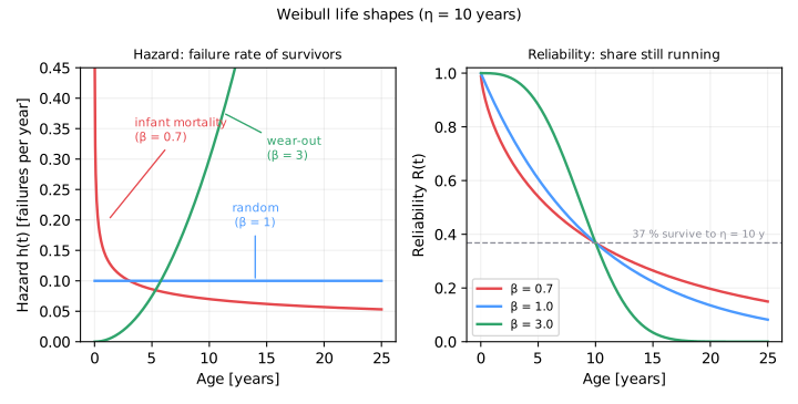
| Shape | Hazard | Physical meaning | Example |
|---|---|---|---|
| \(\beta < 1\) | Falls with age | Infant mortality: defects show early | Electronics after commissioning, poor installs |
| \(\beta = 1\) | Constant | Random: age is irrelevant (exponential) | Lightning, many control faults |
| \(\beta > 1\) | Rises with age | Wear-out | Gearboxes, main bearings, blade erosion |
The hazard turns into a practical question with conditional reliability: given a gearbox has survived to age \(a\), what is the chance it survives one more year?
For a wear-out gearbox (\(\beta = 3\), \(\eta = 12\) years): 98.9 % at age 2, but only 82.6 % at age 10. Same component, same design: the chance of failing in the next year rises from 1.1 % to 17.4 %, about sixteen-fold, with age alone.
β below 1 in a stop log: repeats and bad actors
Fit a Weibull to the time between pitch stops on each turbine of the synthetic farm, and the shape comes out at β ≈ 0.4 (0.36–0.41 depending on how the censored gaps at the ends of the record are treated), close to the ≈ 0.40 in the real event logs. That doesn't mean the pitch systems are getting more reliable with age. Two things produce it:
- Repeats. A reset clears the alarm but not the cause, so the next stop comes soon: short gaps are over-represented.
- Bad actors. Pooling a few turbines that stop often with many that rarely do gives a decreasing hazard even if each turbine's hazard is constant.
The decision it points to is not "replace older pitch systems" but fix it right first time and find the bad actors. Which mechanism dominates is a question for the work orders, not the curve.
Censoring: the turbines that haven't failed are data
Watch a fleet for 12 years. Some gearboxes fail; most are still running. The survivors' lives are right-censored: we know only that they lasted at least 12 years.
The tempting mistake is to fit only the failures. That uses only the short lives,
and badly underestimates life. Weibull.fit(times, failed) maximises the censored
likelihood:
In the test suite, a fleet whose true \(\eta\) is 20 years is fitted correctly with censoring; fitting only the failures gives an \(\eta\) below 14 years. Every fleet reliability study must ask: where are the survivors?
8 · Maintainability: repair time and response
Repair times are lognormal-like: most short, a long tail. On the synthetic farm, pitch-system call-outs that don't wait for parts, including a mean 2-hour technician response, fit a lognormal with median 3.6 h and \(\sigma \approx 1.1\): mean 6.9 h, and only 53 % restored within 4 hours.
The operator has two levers, and the stop log can test both on the same events:
- Response: how quickly a technician reaches a stopped turbine (rostering, on-site technicians, remote reset rights);
- Logistics: how long a stopped turbine waits for a part, a specialist or a crane (spares held on site, service agreements, crane contracts).
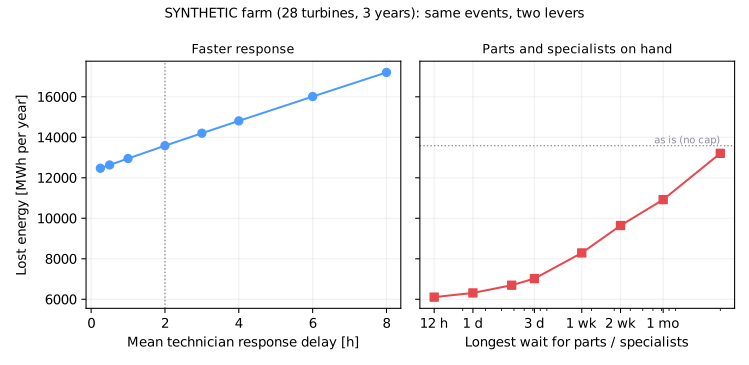
| Mean response delay | Time-based availability | Lost energy (MWh/yr) |
|---|---|---|
| 4 h | 95.37 % | 14,810 |
| 2 h (as is) | 95.70 % | 13,586 |
| 1 h | 95.88 % | 12,953 |
| 0.5 h | 95.96 % | 12,634 |
| Longest wait for parts / specialists | Time-based availability | Lost energy (MWh/yr) |
|---|---|---|
| As is (median wait ≈ 11 days) | 95.70 % | 13,586 |
| 2 weeks | 96.88 % | 9,643 |
| 1 week | 97.35 % | 8,290 |
| 72 h | 97.73 % | 7,023 |
| 24 h | 97.95 % | 6,314 |
At an illustrative $70/MWh, cutting the mean response from 2 h to 0.5 h is worth about 950 MWh, or $67k, per year. Making sure no stopped turbine waits more than 72 hours for a part or a specialist is worth about 6,560 MWh, or $460k, per year, seven times as much, from about 40 outages in three years: one stop in two hundred. Those are the most each arrangement is worth; if it costs more, it doesn't pay, however good the availability chart looks. That is the chapter's recurring question: what decision should change because reliability changed? Chapter 5 turns "parts on site" into a decision about spares, crews and a crane.
9 · The first economic reliability decision: when to replace
The trade-off
A gearbox wears out. Two ways to replace it:
| Planned exchange | Exchange after failure | |
|---|---|---|
| When | Chosen: a calm month, crane booked | Whenever it breaks |
| Cost | Parts + crane | Parts + crane + secondary damage + expediting |
| Outage | ≈ 5 days | ≈ 1–2 months (parts, crane, weather) |
| Lost generation | Low-wind month | Average wind |
Replace too early and you throw away remaining life. Replace too late and you pay for failures.
Decision variable, objective, formulation
The age-replacement policy: replace preventively at operating age \(T\), or on failure if that comes first. By the renewal-reward theorem the long-run cost per hour is
where \(C_p, C_f\) are the total costs of a planned and an unplanned exchange including the value of generation lost (\(D \times v\)), and \(D_p, D_f\) the outage durations. The decision is
One variable, a smooth objective, no constraints: a grid search followed by a bounded scalar optimiser is enough.
from energy_or.reliability import (
    HOURS_PER_YEAR as Y,
    ReplacementCase,
    Weibull,
    optimise_replacement_age,
)

gearbox = ReplacementCase(
    life=Weibull(shape=3.5, scale=12 * Y),
    planned_cost=400e3,
    failure_cost=900e3,
    planned_downtime_h=120,
    failure_downtime_h=1_440,  # 5 days vs 2 months
    planned_lost_value_per_h=56,
    failure_lost_value_per_h=80,
)
print(optimise_replacement_age(gearbox).explain())
All costs, values and life parameters here are illustrative assumptions; only the shape of the outage durations is informed by the real downtime data.
Solve and interpret
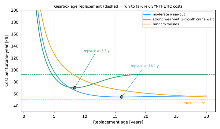
| Case | \(\beta\) | Decision | Cost vs run-to-failure |
|---|---|---|---|
| Random failures | 1.0 | Run to failure | — |
| Moderate wear-out | 2.5 | Replace at 16.1 years | Saves ≈ $1.7k / turbine-yr |
| Strong wear-out, 2-month crane wait | 3.5 | Replace at 8.3 years | Saves ≈ $22k / turbine-yr |
Three lessons:
- No wear-out, no preventive replacement. With \(\beta \le 1\) a new gearbox is no less likely to fail than the old one, so replacing it early only adds cost. The optimiser returns "run to failure", and the test suite checks it for every \(\beta \le 1\).
- Flat optima. For moderate wear-out the cost curve is almost flat: replacing at 12 or 20 years costs nearly the same. When the curve is flat, spend effort on the inputs, not the optimiser.
- Logistics drives the answer. The strong case pays because an unplanned exchange waits two months for a crane, at full lost generation. Shorten that wait (spares, crane contracts, Parts X–XI) and the case for preventive replacement weakens. Reliability, maintainability and logistics are one problem.
10 · Backtest
A real backtest would replay a fleet's history: at each date, fit the life model using only failures and survivors known by then, choose a policy, and compare its realised cost with what actually happened. That requires the information-policy discipline of the backtesting framework (Part XIX). The censoring example in Section 7 is its smallest version: using data available at the time, including survivors, is what separates a sound estimate from a biased one.
11 · Adding realism
- Condition monitoring. Oil debris counts and vibration change the hazard of this gearbox, not the fleet average. Replace age with a health index (Part IX).
- Opportunistic maintenance. If the crane is already on site for one turbine, replacing a second gearbox early is far cheaper (Case C).
- Seasonality. Lost value per hour depends on when the outage happens. The maintenance-window optimiser (Milestone 4) chooses the date, not only the age.
- Spares and crews. With two spare gearboxes and one crane for 100 turbines, individual replacement ages collide. That is a scheduling problem (Case F, MILP).
- Uncertain parameters. Optimise against a distribution of \(\beta\) and \(\eta\), not a point estimate (Part XVII).
12 · Exercises
Guided
A turbine's MTBF is 200 h and MTTR 5 h. Compute its availability. Then halve the MTTR, and separately double the MTBF. Which helps more, and why are they not the same?
Engineering
Fit a Weibull to a fleet where half the turbines were observed for only 5 years. How does the width of the uncertainty on \(\beta\) change? (Hint: bootstrap.)
Market
Lost value per hour depends on price. Re-run the replacement case with
failure_lost_value_per_h doubled (a high-price year). How much does \(T^*\) move?
Challenge
Add a minimal repair option: on failure, repair to "as bad as old" at a lower cost, keeping the age. When does that beat replacement on failure?
Production challenge
The SCADA stop log is reclassified by the O&M contractor every month. Design checks that would detect a silent change in category definitions before it corrupts your failure rates.
13 · Production perspective
- Data first. Stop logs need clean categories, merged chained events (a fault and its repair are one outage), and an agreed rule for common-cause events (a grid undervoltage that stops 16 turbines at once is one event, not 16 failures).
- Report intervals. Every failure rate in a dashboard should carry its exposure and interval.
- Refit on schedule. Life models are re-estimated as survivors age and new failures arrive. Version them, and record which model drove which maintenance decision.
- Feed the economics. Expected revenue is availability × expected generation × value. The maintenance and fleet optimisers that follow consume these models directly.
Run it yourself
| Artefact | Location |
|---|---|
| Reliability models | src/energy_or/reliability/models.py |
| Replacement policy | src/energy_or/reliability/replacement.py |
| Synthetic wind farm | src/energy_or/data/wind_farm.py |
| Tests | tests/test_reliability.py, tests/test_wind_farm.py |
| Animation | animations/reliability/weibull.py |
| Notebook | notebooks/03_reliability.ipynb |