6 · Two farms, two PPAs, one constraint¶

Intermediate Parts V · XIII · XIV · XV Cases A · H · K

In this chapter

Turn a PPA into the value of one more MWh, as a function of the spot price
See why two farms with similar contracts can bid very differently, and why one of them keeps getting constrained off
Understand that the network clears by offer price, while a portfolio should allocate by contract value, and how to make the two agree with a sacrifice band
Discover that a strategy can raise one farm's revenue by 10 % and still lose the portfolio money, because of forecast error next to a contract cliff
Find the one input that decides whether coordination is worth anything

Chapter 1 shared a connection between two farms by value per MWh, as if the owner controlled the allocation. This chapter is the real-world version: the network is shared through a market constraint, the allocation is made by the dispatch process from offers, and each farm's value per MWh comes from its PPA.

Where this case comes from

The contract structures, bidding rules and the coordination strategy follow an operating two-farm portfolio and its operator's own strategy analysis. Capacities are offset, every price is illustrative, and the price data is synthetic.

1 · The real-world problem¶

One owner runs two wind farms behind the same network limit. When it is windy and demand is low, together they can produce more than the network can carry, and prices go negative.

	North	South
Capacity	190 MW	118 MW
PPA	Fixed price, escalating 2.5 %/yr	Fixed price on 95 % of output; 5 % merchant
Illustrative price	$65/MWh	$57/MWh
At negative prices	The farm bears the negative price: it nets price + RRP	Contract pays in full while RRP > −$20; nothing at or below −$20
Lowest permitted offer	Its break-even	−$19.99

South is constrained off again and again. North is not. The operator's question:

Should North deliberately give up some of its dispatch so that South can run?

2 · The physical and market system¶

Behind a binding network constraint, the dispatch process does not ask what each MWh is worth to its owner. It ranks offers by price and fills the limited capacity from the cheapest offer upward. Offers above the regional price aren't dispatched at all.

North can offer down to about −$64.99, the point where its contract stops paying. South may not offer below −$19.99. So whenever the constraint binds, North is always ahead of South in the queue, whatever their contracts are worth.

A simplified clearing model

energy_or.network.offers.clear_offers fills one limit in price order with pro-rata ties. Real dispatch co-optimises the whole region, applies constraint coefficients, loss factors, ramp limits and FCAS, and can produce local prices well below the regional price. This is not NEMDE. It keeps the one mechanism that matters here: offer prices decide who is curtailed.

3 · The decision¶

For each dispatch interval, how should each farm's MW be split across offer prices?

4 · From contract to value per MWh¶

The value of generating one more MWh, as a function of the regional price $RRP$:

\[ v_{North}(RRP) = F_N + \min(RRP, 0) \]

\[ v_{South}(RRP) = 0.95\,F_S\,\mathbb{1}[RRP > -20] \;+\; 0.05\,RRP \;+\; o_S \]

where $F$ is the (escalated) fixed price and $o_S$ is the value of South's minimum-generation obligation: what it costs South, per MWh, to fall short (for example replacing certificates it was contracted to deliver).

Which contracts actually have an $o_S$?

South's real-world counterpart is a government feed-in-tariff style entitlement: the farm transfers every certificate it creates to the counterparty, and each calendar year's certificates are due within three months of year end (by 31 March). It transfers them whether the tariff paid out or not, including for any energy generated at or below the −$20 cliff. Certificates are owed only for energy actually generated, so a MWh South doesn't generate creates no certificate and no debt. That makes $o_S = 0$: the certificates were never South's to sell, and losing a MWh to the constraint costs only the tariff on it. A positive $o_S$ needs a contract with a minimum quantity and a shortfall charge, or a corporate PPA that buys bundled energy and certificates and charges for undelivered certificates.

The same rule explains South's −$19.99 offer. A MWh generated at −$20 earns no tariff, pays the negative price and still hands over its certificate, so South must never be dispatched below the cliff.

Check against the operator's own rule of thumb, with a $62.50 contract price: at $RRP = -\$20$, $v = 62.50 - 20 = \$42.50$/MWh. The test suite asserts exactly this.

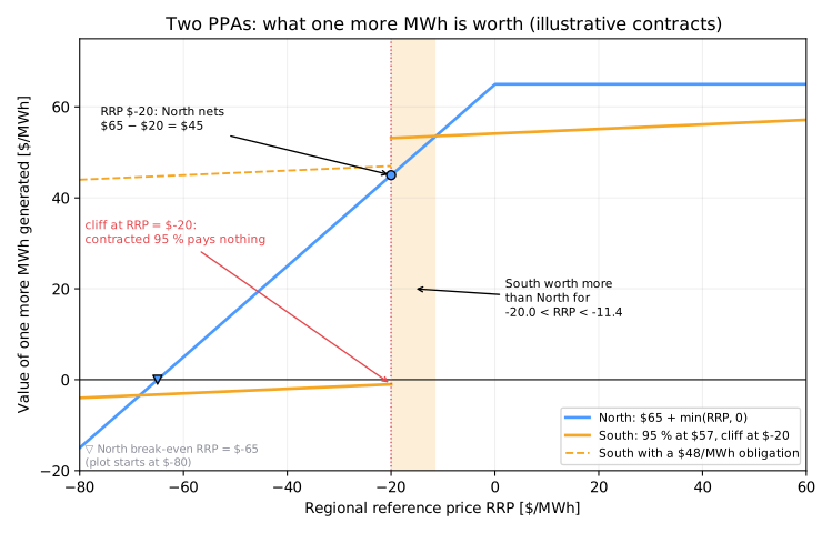
Value per MWh against the regional price

RRP	North	South ($o_S = 0$)	Who is worth more
+$50	$65.00	$56.65	North
$0	$65.00	$54.15	North
−$10	$55.00	$53.65	North
−$15	$50.00	$53.40	South
−$19	$46.00	$53.20	South
−$20	$45.00	−$1.00	North
−$70	−$5.00	−$3.50	Neither should run

Between about −$20 and −$11.40, a South MWh is worth more than a North MWh. Below −$20 South's contract stops paying. That is the cliff.

5 · Objective¶

Maximise the portfolio's value:

\[ \max \sum_t \sum_{f \in \{N, S\}} v_f(RRP_t)\,P_{f,t}\,\Delta t \]

subject to $P_{N,t} + P_{S,t} \le L$, $0 \le P_{f,t} \le \bar P_{f,t}$, and, crucially, the dispatch $P$ is produced by the market from our offers, not chosen directly.

6 · Constraints¶

Constraint	Meaning
$P_N + P_S \le 200$ MW	Shared network limit (both coefficients 1)
$P_f \le \bar P_f$	Available wind
South offers ≥ −$19.99	Contract / operating rule
Dispatch in offer-price order	The market, not the owner, allocates

7 · Formulation: from values to offers¶

Why these techniques? Structure → method¶

Property of the problem	Here	So
Objective	linear in each farm's MW once the price is known: value per MWh × MW	an LP per interval, and Chapter 1's ranking rule solves it
Variables	two continuous MW per 5-minute interval	no integers; but the owner does not set them
Constraints	one shared-limit row, $P_N + P_S \le 200$, both coefficients 1, plus two bounds	a one-row knapsack: fill the limit in order of value (no slack, surplus or artificial variables are needed in a hand solution)
Who decides	the market clears by offer price, not by value	the owner's real variables are offer prices and band volumes: a bid-design problem
Time coupling	none: each interval is independent (no storage)	solve interval by interval; a week is 2,016 separate small problems
Information	the price at dispatch is unknown; the bid is set on a forecast with about $12/MWh error	decide on the expected value, not on the point forecast
Non-convexity	South's value drops to zero at −$20, a cliff	the value function is not concave; check it by simulation, not by theory alone

Chosen. - Ranking by value per MWh is the exact solution of the one-row LP. With a single coupling constraint and unit coefficients, filling the limit from the highest value down is the LP optimum, so no solver is needed to know what the market should do. - Sacrifice bands translate that ranking into offers. The market allocates by offer order, so the higher-value farm offers low and the other farm's displaced MW sit one cent behind it. - Expected value under forecast error (the risk-aware policy) replaces the point forecast, because a cliff next to the forecast makes a point forecast dangerous.

Not chosen. - A direct allocation LP (Chapter 1's model). It is the right answer to "what should dispatch be?", but the owner cannot set dispatch. Using it alone would hide the problem of this chapter. - A bilevel model of the market (owner above, clearing below). It is the general tool for optimal offers, but it needs the clearing engine's full rules, and the book does not reproduce NEMDE. A one-cent rule captures the mechanism that matters. - A scenario-based stochastic programme. With one price per interval, the expectation over forecast error is a one-line integral, so scenarios add cost without insight.

What the theory guarantees. - If the offers sort the farms in value order, clearing reproduces the LP optimum for that interval. The guarantee holds only for the price the offers were built on: across a cliff the ranking can be wrong, which is why the point-forecast policy can lose money while the risk-aware one never does worse than local bidding here.

References. - Stoft (2002), Power System Economics: what an offer does to dispatch and price, and why bidding at cost is not always best (Chapter 6). - Biggar and Hesamzadeh (2014), The Economics of Electricity Markets: congestion and constrained-off generation behind a shared limit (Chapter 6). - Bertsimas and Tsitsiklis (1997), Introduction to Linear Optimization: why the optimum of a one-row LP sits at a corner (Chapter 1). - Choosing a technique for how structure picks the method.

If the owner could allocate directly, this would be Chapter 1's LP: give the limit to the higher-value farm first. The owner can't, so the job is to design offers that make the market reproduce the LP's answer:

Rank the farms by value per MWh at the expected price.
The higher-value farm offers its MW at its own low price.
Any MW of the lower-value farm that would push the higher-value farm out are offered one cent above the higher-value farm's offer, a sacrifice band. They are dispatched only if the network turns out to have room.

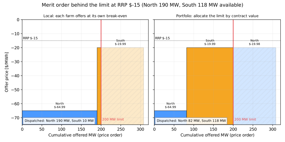
When South is worth more (RRP between −$20 and −$11.40), North's displaced MW go in at −$19.98, one cent above South's −$19.99.

from energy_or.contracts import local_offers, portfolio_offers
from energy_or.data.contracts import NORTH, SOUTH, SHARED_LIMIT_MW
from energy_or.network.offers import clear_offers

local = local_offers([NORTH, SOUTH], [190, 118])
shaped = portfolio_offers([NORTH, SOUTH], [190, 118], SHARED_LIMIT_MW, rrp_forecast=-15)
clear_offers(shaped, SHARED_LIMIT_MW, rrp=-15)  # {'North': 82, 'South': 118}

8 · Visualisation¶

Offer stacks at RRP −$15: local versus portfolio offers

9 · One interval, by hand¶

Both farms fully available (190 + 118 MW), limit 200 MW, $RRP = -\$15$:

Offers	North MW	South MW	North value	South value	Portfolio $/h
Each at its own price	190	10	$9,500	$534	$10,034
Portfolio (sacrifice band)	82	118	$4,100	$6,301	$10,401

Coordinating is worth $367 per hour in this interval. South's revenue jumps about twelve-fold; North's falls by more than half. Most of South's gain is a transfer from North, and the portfolio keeps only the difference in value per MWh (about $3.40 × 108 MW).

10 · Solve: a synthetic week¶

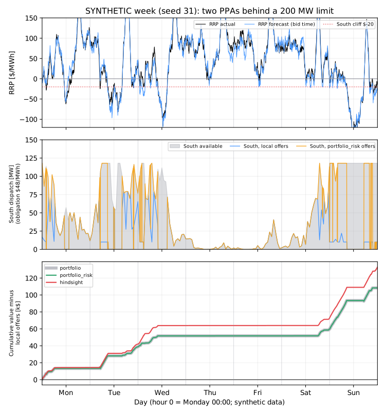
Simulate every 5-minute interval of a synthetic week (seed 31) under four policies. Prices are synthetic and fall when it is windy, so negative prices and the binding constraint arrive together. The constraint binds in 37 % of intervals, prices are negative in 25 %, and under local bidding South is curtailed for 65 % of its available energy against North's 11 %.

Policy	How offers are made
Local	Each farm offers all its MW at its own break-even
Portfolio	Sacrifice bands chosen from a point price forecast
Portfolio, risk-aware	Farms ranked by expected value given the forecast's error
Hindsight	The same rule with the actual price: an unreachable bound

The price forecast available at bidding time has an error of about $12/MWh, with persistence: predispatch is often wrong in the same direction for a while.

A synthetic week: prices, South's dispatch, cumulative gain

11 · Interpret¶

Without an obligation, coordination is worth almost nothing¶

Averaged over three synthetic weeks, against local bidding (about $890k/week):

South's obligation $o_S$	Portfolio (point forecast)	Portfolio (risk-aware)	Hindsight bound
$0/MWh (South's actual structure)	−$2,150	+$6	+$1,156
$20/MWh	+$18,666	+$18,666	+$28,154
$48/MWh	+$70,950	+$70,950	+$86,980

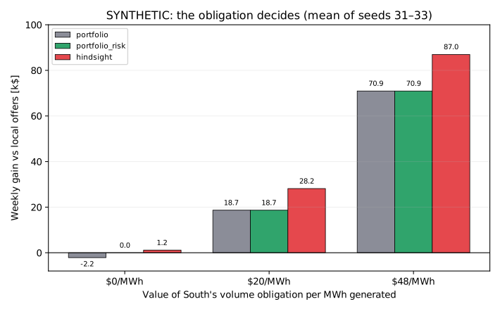
Weekly gain from coordination against South's obligation value

With $o_S = 0$ the sacrifice strategy raises South's revenue by about 10 % and lowers the portfolio's value. Three reasons:

The window is narrow. South is worth more only between −$20 and −$11.40, and only matters when the constraint binds: about 3 % of intervals.
The margin is thin. In that window South beats North by at most about $8/MWh.
The cliff is next door. Sacrifice when the forecast says −$15, and if the price lands at −$22, South's −$19.99 offer doesn't clear, North's sacrificed MW at −$19.98 don't either, and the portfolio earns $3,526/h instead of $8,170/h.

The point-forecast policy takes that gamble every time. The risk-aware policy computes South's expected value given the forecast error,

\[ \mathbb{E}[v_S] = 0.95\,F_S\,\Pr(RRP > -20) + 0.05\,\mathbb{E}[RRP] + o_S , \]

and stops sacrificing when the cliff is close. It never loses to local bidding, and here it never gains much either.

The obligation decides¶

If each MWh South fails to generate costs it money, for example certificates it must replace or a generation guarantee it must meet, South's value per MWh rises by that amount, and coordination becomes worth 2–8 % of the portfolio's value. The decision to coordinate rests on one number the trading model can't invent: what South's PPA actually charges for a shortfall, and whether network curtailment is excused.

For the contract South is modelled on, the answer is nothing. Its certificate transfer is owed only on energy actually generated, as described in §4, so $o_S = 0$ and the first row of the table applies. Sacrificing North doesn't pay; at best, the risk-aware policy roughly breaks even. The $20 and $48 rows are not hypothetical in general, because many corporate PPAs carry shortfall charges, but they are not South's case. Read the contract before writing the bidding strategy.

The lesson

Locally optimal bidding (each farm at its own break-even) and portfolio-optimal bidding differ only when the contracts disagree with the merit order. Whether the difference is worth chasing depends on (1) how often the constraint binds in the disputed price range, (2) the value gap per MWh, (3) forecast error near any contract cliff, and (4) obligations that make lost MWh expensive. A strategy that raises one asset's revenue can still destroy portfolio value.

12 · Backtest¶

This chapter's week is synthetic and its forecast error is invented. A real backtest would replay archived predispatch forecasts and dispatch outcomes, apply the offers each policy would have submitted at the time, and value the result with the real contracts, including South's actual shortfall terms. That is Milestone 7, and this chapter's policies are already written to plug into it.

13 · Adding realism¶

Rebidding. Offers can be changed close to real time as predispatch updates; the forecast error at the last rebid is smaller than a day ahead.
Constraint coefficients and local price. Real constraint equations weight each unit; the farm with the larger coefficient loads the limit more per MW (Chapter 1).
Escalation. Both contract prices escalate, so the crossover price drifts year by year; the notebook tracks it.
Annual obligations. A volume obligation that bites only if the year's output falls short is a stochastic, intertemporal problem: a MWh lost in a windy March may cost nothing by December (Part XVII). An annual certificate transfer (each year's certificates by 31 March) is not one of these. It is settlement of what was generated, a cash-flow and compliance date rather than a reason to generate.
Separate financing. If the two farms have separate lenders, a dollar is worth more to the one closer to its covenants, and coordination can pay even with no obligation: Chapter 7.
More units. Other generators behind the same constraint, with their own offers, turn this into a game (Part V).

14 · Exercises¶

Guided

At RRP −$15, both farms full, compute the portfolio's $/h for local and portfolio offers by hand. Then repeat at −$5 and at −$25.

Engineering

Give North a constraint coefficient of 0.8 and South 1.0. How does the value-per-MW- of-limit ranking change?

Market

Raise South's cliff to −$10. What happens to the sacrifice window and to the value of coordination?

Challenge

Replace the per-interval obligation value with an annual volume obligation and a shortfall price. Formulate the year as a stochastic programme: when is it worth keeping South running in March?

Production challenge

The sacrifice band is a rebid decision taken every 5 minutes on predispatch. Design the guardrails: when must the system not sacrifice (forecast close to the cliff, stale predispatch, missing data), and what does it log so a trader can audit each decision?

15 · Production perspective¶

Contracts as code. Encode each PPA's settlement, cliff, shares and obligations as tested functions, with the clause reference in the docstring. Here, a wrong sign at the cliff costs real money.
Bid with uncertainty. Use the predispatch price distribution, not the point forecast, whenever a decision sits next to a contract cliff.
Measure the portfolio, not the asset. Report value per farm and for the portfolio, so a 10 % gain for one farm is never mistaken for a gain overall.
Respect the rules. Offers must follow the market's bidding and rebidding rules and each contract's terms; the optimiser only chooses among permitted offers.

Run it yourself¶

Artefact	Location
PPA value models	`src/energy_or/contracts/ppa.py`
Offer policies and simulation	`src/energy_or/contracts/bidding.py`
Price-ordered clearing	`src/energy_or/network/offers.py`
Synthetic farms and week	`src/energy_or/data/contracts.py`
Tests	`tests/test_contracts.py`
Animation	`animations/contracts/offer_stack.py`
Notebook	`notebooks/06_two_ppas_one_constraint.ipynb`

Constraint	Meaning
\(P_N + P_S \le 200\) MW	Shared network limit (both coefficients 1)
\(P_f \le \bar P_f\)	Available wind
South offers ≥ −$19.99	Contract / operating rule
Dispatch in offer-price order	The market, not the owner, allocates